Suppose you have a fixed budget for cloud instances. Each instance has a cost and a throughput value, and you must either take it or leave it. Trying every combination repeats many of the same smaller calculations. A two-dimensional matrix lets you save those results instead: rows represent how many items you may consider, and columns represent capacities from zero up to your budget. section 7.1
For n items and capacity W, make a grid with (n + 1) rows and (W + 1) columns. A cell T[i, w] holds the best value achievable using the first i items within capacity w. Fill the row for zero items and the column for zero capacity with zeroes. Then work across each item row, using values already recorded in the previous row. section 7.1
To fill a cell, ask whether the current item fits:
- If it does not fit, copy the value directly above: you cannot take it. section 7.1
- If it fits, compare the value above (skip it) with its value plus the previous row's result at the remaining capacity (take it). Record the larger value. Looking at the previous row prevents you from taking the same item twice. section 7.1
A small budget decision
Say the first instance costs 1 credit and gives value 2; the second costs 2 credits and gives value 3. At capacity 3, cell T[2, 3] compares skipping the second instance, worth T[1, 3] = 2, with taking it, worth 3 + T[1, 1] = 5. Write 5. With four instances and a capacity of 8, the completed grid ends at T[4, 8] = 11: taking the fourth instance gives 6 + T[3, 3] = 11, beating the value 10 from skipping it. section 7.1
Figure 7.3 Visualization of the math used to evaluate cell T[2, 3] (circled in green) on the second row (w2 = 2, v2 = 3). The algorithm resolves a binary choice by executing a maximum value comparison between two paths. The exclusion path inherits the value directly above (T[1, 3] = 2). The active inclusion path accepts the new instance's throughput value (v2 = 3, highlighted in the red solid box) and subtracts its weight from the current capacity (3 - 2 = 1), forcing a pointer lookup to the previous row at column 1 (T[1, 1] = 2, highlighted by the red dotted circle). The combined value of 5 outperforms the exclusion path, updating the cell state.
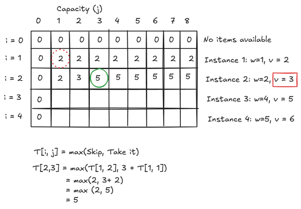
Follow the arrows from T[2, 3] to see both choices draw on the previous row, including the lookup at the capacity left after taking the item. section 7.1
The full grid makes past decisions easy to inspect, but it takes O(n × W) time and O(n × W) space. Because each new row depends only on the preceding row, a one-dimensional array can reduce memory use when updated appropriately. The grid is useful for indivisible, 0/1 choices; when items can be divided, fractional knapsack instead permits a greedy strategy. section 7.3 section 7.3