Maximum a posteriori (MAP) estimation chooses the parameter value θ that is most probable after observing data X: it maximizes the posterior p(θ|X). By Bayes’ theorem, the denominator does not depend on θ, so MAP maximizes p(X|θ)p(θ): the likelihood supplied by data times a prior encoding beliefs about parameter values. section 6.6.3 section 13.11
MAP differs from maximum likelihood estimation (MLE) by retaining the prior. MLE maximizes p(X|θ) alone; MAP adds p(θ), favoring parameters with an expected property while still fitting observations. A prior proportional to e^(−||θ||²), for example, favors smaller parameter magnitudes, making MAP equivalent to regularized MLE. section 6.10 section 6.6.1
The balance between evidence and belief changes with the amount of data:
- With little data, the prior can substantially determine the posterior and compensate for missing evidence. section 13.1.1
- With abundant data, the likelihood increasingly dominates, and MAP approaches the MLE estimate. section 13.6.1
- A weak prior is easily overwhelmed by data; a strong prior resists it. section 13.11
Gaussian parameter fitting with regularization
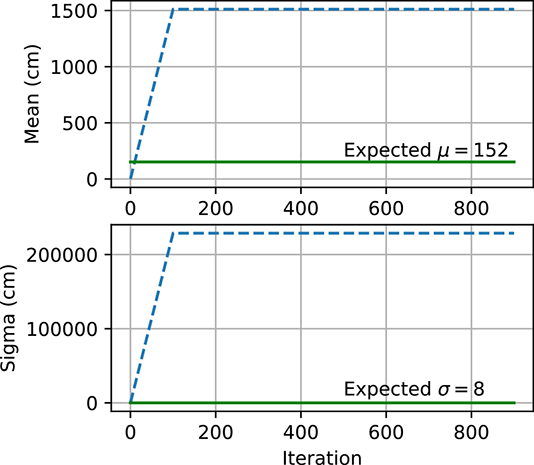
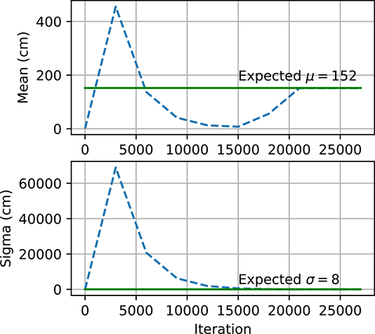
For Gaussian data, gradient-based MLE can produce very large μ and σ when initialized far from expected values. A MAP loss adds squared μ and σ penalty terms to the negative log-likelihood. In the illustrated run, this regularization lets the estimates converge from a distant initialization. section 6.8.2 section 6.8.2
MAP can also be read as selecting the mode of a computed posterior distribution. With a Gaussian likelihood and Gaussian prior over an unknown mean, the posterior is Gaussian and its mean μn is the MAP estimate. For unknown precision with a gamma posterior, the MAP precision is (αn−1)/βn. section 13.3 section 13.6.1
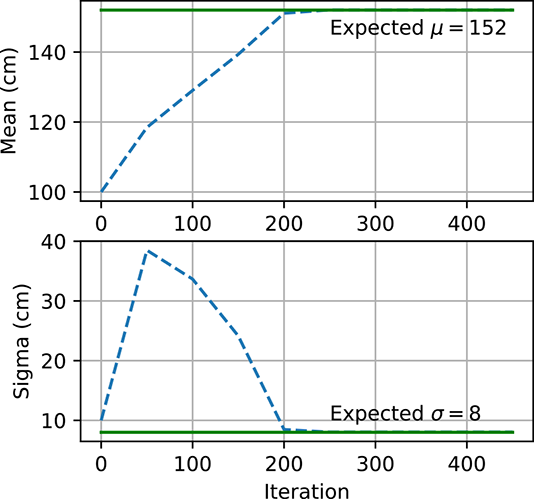
Figure 6.5 Gaussian parameter estimation using maximum likelihood estimate and maximum a posteriori estimation. In figure 6.5a, the MLE explodes because μ and σ are initialized far from μexpected and σexpected. However, the MLE converges in figure 6.5b because μ and σ are initialized closed to μexpected and σexpected. Figure 6.5c shows how, for MAP, μ and σ are able to converge to μ.expected and σexpected even though they are initialized far away.
|
(a) MLE explodes: μinit = 1, σinit = 1. |
|
(b) MLE converges: μinit = 100, σinit = 10. |
|
(c) MAP converges: μinit = 1, σinit = 1. |
Compare MLE and MAP optimization trajectories for Gaussian mean and standard deviation under near and far initializations. section 6.8.2
