Mean-field approximation makes variational inference tractable by replacing a joint posterior p(x₁,…,xₙ) with a fully factorized distribution q(x) = ∏ᵢ qᵢ(xᵢ). Each factor has its own parameters. The factors are independent in q, even when the variables interact in the probability model. section 3.2
Figure 3.3 True posterior (left), structured approximation (middle), and fully factored approximation (right)
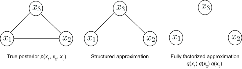
Compare the true posterior, a structured approximation, and the fully factored approximation to see what the mean-field assumption removes. section 3.2
Choose the factors by minimizing variational free energy, or equivalently maximizing the evidence lower bound (ELBO). Hold all factors except qⱼ fixed and optimize qⱼ. Its update depends on an expectation over the other factors: their uncertain values enter through their current means. Repeating these updates turns joint-posterior approximation into an iterative optimization procedure. section 3.2 section 3.0
Denoising a binary image
Let each hidden pixel xᵢ be −1 or +1, and let its noisy observation yᵢ be Gaussian with mean xᵢ and variance σ². In an Ising model, a positive coupling J favors neighboring pixels with the same state. Approximate the hidden image with one binary factor qᵢ(xᵢ) per pixel, parameterized by its mean μᵢ. For each update, combine the local observation with the weighted means of neighboring pixels, then recompute μᵢ. A learning rate λ between 0 and 1 controls how far the parameter moves toward its new value; the ELBO can be tracked across iterations. section 3.3
Listing 3.1 Mean-field variational inference in an Ising model
import numpy as np
import pandas as pd

import seaborn as sns
import matplotlib.pyplot as plt

from PIL import Image
from tqdm import tqdm
from scipy.special import expit as sigmoid
from scipy.stats import multivariate_normal

np.random.seed(42)
sns.set_style('whitegrid')

class image_denoising:

    def __init__(self, img_binary, sigma=2, J=1):

        #mean-field parameters
        self.sigma  = sigma    #1
        self.y = img_binary + self.sigma*np.random
         .randn(M, N)     #2
        self.J = J    #3
        self.rate = 0.5   #4
        self.max_iter = 15
        self.ELBO = np.zeros(self.max_iter)
        self.Hx_mean = np.zeros(self.max_iter)

    def mean_field(self):

        #Mean-Field VI
        print("running mean-field variational inference...")
        logodds = multivariate_normal.logpdf(self.y.flatten(), mean=+1,
         cov=self.sigma**2) - \
                  multivariate_normal.logpdf(self.y.flatten(), mean=-1,
                   cov=self.sigma**2)
        logodds = np.reshape(logodds, (M, N))

        #init
        p1 = sigmoid(logodds)
        mu = 2*p1-1    #5

        a = mu + 0.5 * logodds
        qxp1 = sigmoid(+2*a)  #q_i(x_i=+1)
        qxm1 = sigmoid(-2*a)  #q_i(x_i=-1)

        logp1 = np.reshape(multivariate_normal.logpdf(self.y.flatten(),
         mean=+1, cov=self.sigma**2), (M, N))
        logm1 = np.reshape(multivariate_normal.logpdf(self.y.flatten(),
         mean=-1, cov=self.sigma**2), (M, N))

        for i in tqdm(range(self.max_iter)):
            muNew = mu
            for ix in range(N):
                for iy in range(M):
                    pos = iy + M*ix
                    neighborhood = pos + np.array([-1,1,-M,M])
                    boundary_idx = [iy!=0,iy!=M-1,ix!=0,ix!=N-1]
                    neighborhood = neighborhood[np.where(boundary_idx)[0]]
                     xx, yy = np.unravel_index(pos, (M,N), order='F')
                    nx, ny = np.unravel_index(neighborhood, (M,N), order='F')

                    Sbar = self.J*np.sum(mu[nx,ny])
                    muNew[xx,yy] = (1-self.rate)*muNew[xx,yy] +
                     self.rate*np.tanh(Sbar + 0.5*logodds[xx,yy])
                    self.ELBO[i] = self.ELBO[i] + 0.5*(Sbar * muNew[xx,yy])
                #end for
            #end for
            mu = muNew

            a = mu + 0.5 * logodds
            qxp1 = sigmoid(+2*a) #q_i(x_i=+1)
            qxm1 = sigmoid(-2*a) #q_i(x_i=-1)
            Hx = -qxm1*np.log(qxm1+1e-10) - qxp1*np.log(qxp1+1e-10) #entropy

            self.ELBO[i] = self.ELBO[i] + np.sum(qxp1*logp1 + qxm1*logm1)
             + np.sum(Hx)
            self.Hx_mean[i] = np.mean(Hx)
        #end for
        return mu

if __name__ == "__main__":

    #load data
    print("loading data...")
    data = Image.open('./figures/bayes.bmp')
    img = np.double(data)
    img_mean = np.mean(img)
    img_binary = +1*(img>img_mean) + -1*(img<img_mean)
    [M, N] = img_binary.shape

    mrf = image_denoising(img_binary, sigma=2, J=1)
    mu = mrf.mean_field()

    #generate plots
    plt.figure()
    plt.imshow(mrf.y)
    plt.title("observed noisy image")
    plt.show()

    plt.figure()
    plt.imshow(mu)
    plt.title("after %d mean-field iterations" %mrf.max_iter)
    plt.show()

    plt.figure()
    plt.plot(mrf.Hx_mean, color='b', lw=2.0, label='Avg Entropy')
    plt.title('Variational Inference for Ising Model')
    plt.xlabel('iterations'); plt.ylabel('average entropy')
    plt.legend(loc='upper right')
    plt.show()

    plt.figure()
    plt.plot(mrf.ELBO, color='b', lw=2.0, label='ELBO')
    plt.title('Variational Inference for Ising Model')
    plt.xlabel('iterations'); plt.ylabel('ELBO objective')
    plt.legend(loc='upper left')
    plt.show()
The implementation shows the iterative mean-field denoising procedure, including its noise, coupling, learning-rate, and ELBO settings. section 3.3
