The Michalewicz function is a nonconvex benchmark with multiple local minima, making it useful for testing optimization algorithms. In two dimensions, its minimum is −1.8013 near (2.20, 1.57), with m usually set to 10. section 9.2.4
A particle swarm optimization implementation typically:
- Evaluates single positions and batches by reshaping one-dimensional inputs into two-dimensional arrays. section 9.2.4
- Stores each particle’s position, velocity, personal-best position, and personal-best value. section 9.2.4
- Updates velocity from inertia, cognitive attraction toward the personal best, and social attraction toward the global best. section 9.2.4
- Searches the two-dimensional domain [0, π] using swarm size, iteration count, and PSO coefficients. section 9.2.4
Two-dimensional PSO result
With 50 particles, 1,000 iterations, and options w = 0.9, c1 = 0.5, and c2 = 0.3, a from-scratch solver returns approximately [2.183, 1.570] with value −1.8013. pymoo and PySwarms produce similarly close solutions near [2.203, 1.571]. section 9.2.4
Listing 9.1 Solving the Michalewicz function using PSO
import numpy as np
import math
import matplotlib.pyplot as plt

def michalewicz_function(position):
    m = 10
    position = np.array(position)
    if len(position.shape) == 1:            #1
        position = position.reshape(1, -1)  #1
    n = position.shape[1]
    j = np.arange(1, n + 1)
    s = np.sin(position) * np.power(np.sin((j * np.square(position)) /
 np.pi), 2 * m)                           #2
    return -np.sum(s, axis=1)               #2
#1 Reshape to a 2D array with a single row if the position is a size-1 array.
#2 The Michalewicz formula
Use the Python listing to inspect the formula and its batch-compatible NumPy implementation. section 9.2.4
Figure 9.6 3D and 2D plots of the Michalewicz function. The three solutions are all very close to the optimal solution.
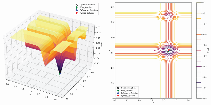
Use the plots to compare the function’s surface and nearby solutions. section 9.2.4
