A model can fit every training example and still explain little: it may simply memorize noise. Minimum description length (MDL) offers a different test. Prefer the explanation that uses the fewest bits to describe both the model and the data encoded with it. A better fit is worthwhile only when the bits it saves outweigh the bits needed for the added complexity. section 8.3 section 8.4.1
Three sequences of 10,000 bits
Peter Grünwald contrasts a repeated pattern, a sequence of coin flips, and a sequence with roughly four times as many 0s as 1s. “0001 × 2500” describes the first compactly. The coin flips offer no discernible pattern to exploit. The biased sequence falls between them: its statistical regularity helps compress it, even without a fixed repeating pattern. Compression is evidence that an explanation has captured structure. section 8.3
MDL makes simplicity a practical model-selection rule rather than a demand for the shortest imaginable explanation. It is connected to Kolmogorov complexity, but works within a chosen class of models; patterns that class cannot represent remain out of reach. Within that limit, charging for complexity discourages a model from spending many bits to fit training noise. section 8.3
Figure 8.6 A simple polynomial (left) underfits the data, a complex polynomial (middle) can achieve zero training error but wastes bits describing noise, and a tradeoff polynomial (right) identifies the broad trend without including the noise. Used with permission granted by the lead author (Peter Grünwald).
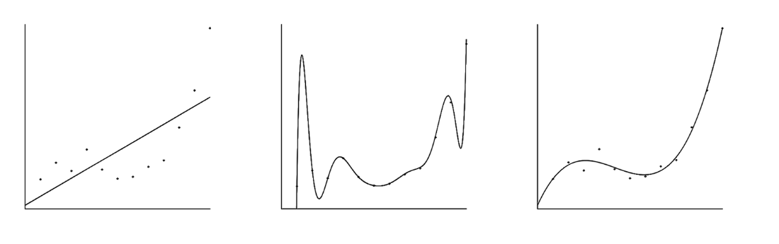
The polynomial comparison makes the trade-off visible: a simple curve misses the trend, an elaborate curve fits the noise, and an intermediate curve captures the broad pattern without paying to describe every fluctuation. section 8.3
Geoffrey Hinton and Drew van Camp turned this principle into a neural-network training objective: minimize the bits needed to specify the weights plus the bits needed to encode prediction errors. They treated each weight as a Gaussian random variable and used a Kullback–Leibler divergence term to measure weight complexity in bits. Allowing a weight more variability makes it cheaper to describe but can hurt accuracy; specifying it more precisely can improve fit at a higher bit cost. section 8.4.1
In a peptide activity prediction test with 105 training examples, their MDL-regularized network achieved 0.286 relative test error, against 0.967 without the MDL term and 0.317 for carefully tuned weight decay. The result showed the value of the trade-off on a small dataset, not a universal win: the implementation required difficult gradient calculations, the evaluation was preliminary, and simpler regularizers could often deliver similar results with less work. The enduring lesson is pragmatic—fit matters, but so does what must be specified to obtain it. section 8.4.2 section 8.4.3
