Imagine customers with several distinct spending patterns. One bell-shaped curve may miss those groups, but a mixture can give each pattern its own curve. A mixture weight says how prevalent each group is: a larger weight gives its curve a larger contribution to the overall distribution. section 8.1
For components with densities f₁(x), f₂(x), and so on, the mixture density at x is w₁f₁(x) + w₂f₂(x) + ⋯. Each weight wₖ is between 0 and 1, and all the weights sum to 1. A component also has its own center and spread; its weight describes prevalence, not location or width. Mixtures can combine distributions other than Gaussians. section 8.1
Learning two weights
Suppose waiting times show a short-wait group and a long-wait group. Model their two weights as unknown quantities rather than fixing their sizes in advance. A Dirichlet prior models weights jointly while keeping them nonnegative and summing to 1. For just two groups, a beta prior on one weight is another option: the second weight is one minus the first. In PyMC, `pm.Dirichlet("w", np.ones(2), dims="cluster")` sets a uniform prior over the two weights. section 8.4 section 8.5
A weight describes a group's overall prevalence, not the chance that any particular observation belongs to it. For an observed value x, multiply each component's density at x by its weight, then divide each weighted density by their sum. This yields a membership probability for each group: a less prevalent group can still be a strong match for a particular value. section 8.8
Take care when reading fitted weights. In a symmetric mixture, component labels can swap between posterior samples: the short-wait group's weight may appear as either w₁ or w₂. Ordering clusters by their centers gives the labels a consistent interpretation. If the number of groups is uncertain, a stick-breaking process can generate weights from successive portions of a unit-length stick; in a truncated model, components with negligible weights can effectively be ignored. section 8.7 section 8.9 section 8.10
Figure 8.11 The average weights of individual components in the mixture, averaged across posterior samples. Only the first 2 components have non-negligible weights.
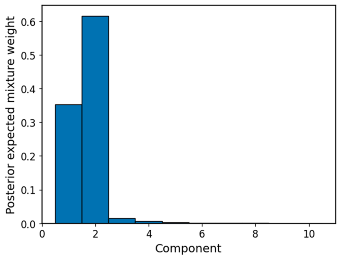
The plotted average weights show a practical distinction: a model can allow ten components while assigning appreciable weight to only two. section 8.10


