Monte Carlo integration estimates an integral by averaging function values at random samples rather than evaluating the function on a fixed grid. Sampling concentrates computation where probability is nonnegligible, making the approach useful for high-dimensional problems. section 2.2 section 2.9
For an integral over an interval, the basic construction is:
- Draw samples from a uniform distribution on (a, b), whose density is 1/(b − a). section 2.2
- Evaluate the integrand at each sample and average the scaled values w(x) = f(x)(b − a). section 2.2
- Increase the sample count N to improve accuracy; the standard error decreases as σ/√N, with σ the empirical standard deviation. section 2.2
Estimating π with random points
Sample points uniformly from a square spanning −R to R in both coordinates. Use the indicator x² + y² ≤ R² to identify points inside the circle, estimate the circle's area from the average indicator contribution, and divide by R². A 10,000-sample implementation reports π = 3.1348 ± 0.0164. section 2.2
Figure 2.4 Pi estimator pseudo-code
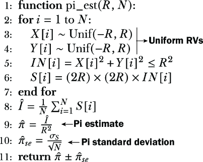
Use the estimator pseudocode to follow sampling, inside-circle testing, area estimation, and normalization. section 2.2
Listing 2.1 Pi estimator
import numpy as np
import matplotlib.pyplot as plt

np.random.seed(42)     #1

def pi_est(radius=1, num_iter=int(1e4)):     #2


    X = np.random.uniform(-radius,+radius,num_iter)
    Y = np.random.uniform(-radius,+radius,num_iter)

    R2 = X**2 + Y**2
    inside = R2 < radius**2
    outside = ~inside

    samples = (2*radius)*(2*radius)*inside

    I_hat = np.mean(samples)
    pi_hat = I_hat/radius ** 2     #3
    pi_hat_se = np.std(samples)/np.sqrt(num_iter)    #4
    print("pi est: {} +/- {:f}".format(pi_hat, pi_hat_se))

    plt.figure()
    plt.scatter(X[inside],Y[inside], c='b', alpha=0.5)
    plt.scatter(X[outside],Y[outside], c='r', alpha=0.5)
    plt.show()

if __name__ == "__main__":

    pi_est()
Use the complete Python implementation to reproduce the estimate, standard error, and inside/outside sample plot. section 2.2
