Newton-raphson method

As explained in Ensemble Methods for Machine Learning

Newton's method is an iterative optimization method that uses first- and second-derivative information to choose updates toward a local minimum.

The Newton-Raphson method, also called Newton’s descent for minimization, is an iterative optimizer that moves model parameters toward a local minimum. Like gradient descent, it repeatedly updates a current estimate. Its distinguishing feature is curvature: it uses both the gradient, or first derivative, and the Hessian, or second-derivative matrix, to choose a more informative next step. section 6.1

Figure 6.1 Comparing gradient descent (left) and Newton’s method (right). Gradient descent only uses local first-order information near the current solution, which leads to a linear approximation of the function being optimized. Different step lengths will then lead to different next steps. Newton’s method uses both local first- and second-order information near the current solution, leading to a quadratic (parabolic) approximation of the function being optimized. This provides a better estimate of the next step.

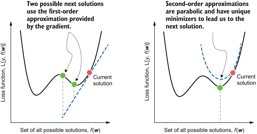
Compare the local approximations: gradient descent follows a linear view of the loss, whereas Newton’s method uses a quadratic view that can estimate a better step. section 6.1

At parameters w, compute the gradient g and Hessian H. The Newton direction is -H⁻¹g, and the update adds that direction to w. In the idealized method, the step length is 1, so no separate step-length search is needed. The Hessian adjusts the gradient using local curvature, which can make the path to a minimum more direct and convergence faster than first-order gradient descent. section 6.1 section 6.1.1

A practical Newton-Raphson loop is:

• Start from an initial parameter guess. section 6.1.1
• Evaluate the loss gradient and Hessian at the current estimate. section 6.1.1
• Form the negated Hessian-inverse gradient direction and take the update. section 6.1.1
• Test whether consecutive estimates differ by less than a chosen tolerance; otherwise repeat. section 6.1.1

Finding a minimum of the Branin function

For the two-variable Branin function, Newton’s method computes an analytic gradient and Hessian, begins at [2, -5], and follows a path toward one local minimum. Compared with gradient descent from the same start, the Newton path is more direct because each update uses a second-order local approximation. A zero gradient is not sufficient to guarantee a minimum, however: descent methods can also converge to a saddle point. section 6.1.1

Training a linear classifier

Newton’s descent can minimize a squared-loss objective for a 2D binary classifier. The loss gradient and Hessian are derived from the training matrix, then used to learn the weight vector. On the illustrated nearly linearly separable data, Newton’s descent reaches a model similar to gradient descent’s in 12 iterations rather than 20, with reported training accuracy of 0.995. section 6.1.2 section 6.1.2

Newton’s method supplies the optimization intuition behind Newton boosting. Rather than directly computing one overall Newton update, Newton boosting learns weak estimators from per-example gradient residuals and Hessian information. This avoids directly computing an expensive full gradient or Hessian while approximating Newton-style updates; the boosting version uses a learning rate rather than relying on an exact unit step. section 6.2.1 section 6.1

Second-order information is valuable when curvature improves the step estimate, but it comes with a cost: computing a Hessian can be computationally expensive. In tree-based Newton boosting, weighted residuals combine gradient-derived residuals with Hessian-derived weights to emphasize badly misclassified examples, and regularized objectives, learning rates, and early stopping help control overfitting. section 6.2.1 section 6.6

How Ensemble Methods for Machine Learning covers it

How deep it goes

Derives gradient-and-Hessian updates, gives convergence pseudocode, and implements optimization for Branin and squared-loss classification.

Examples

Uses the Branin function, a saddle point, and a synthetic two-class squared-loss linear classifier.

What it assumes

Reinforces gradients, loss minimization, matrices, and Hessians while assuming familiarity with gradient descent and linear classification.

What you can do after

Build it from scratch by computing gradients and Hessians, applying Newton updates, and stopping when parameter changes meet a tolerance.

How it connects

Connects gradient descent, Hessian matrices, loss functions, Newton boosting, gradient boosting, AdaBoost, XGBoost, and regularization.

liveBookmanning.com

Read Ensemble Methods for Machine Learning on liveBook Get the book at manning.com

Also explained in

• 

  liveBookmanning.com
  Machine Learning for Tabular Data: XGBoost, Deep Learning, and AIA Newton-Raphson update is an optimization step that uses first- and second-order derivatives to refine parameter values.

Compare how 2 books explain newton-raphson method →

Related concepts

• gradient descentcontrasts with · Gradient descent is an iterative optimization method that updates parameters opposite the gradient of an objective function to reduce its value.
• Hessian matrixuses · A Hessian matrix is the square matrix of second-order partial derivatives of a scalar-valued multivariable function, describing its local curvature.
• Newton boostingused by · Newton boosting is a boosting approach that uses first- and second-order loss information to construct successive learners.
• second-order optimizationkind of · Second-order optimization is an optimization approach that uses first-derivative information together with curvature information, such as a Hessian or its approximation.
• quadratic approximationused by · A quadratic approximation estimates a function locally using terms through second order, including its value, first derivative, and second derivative.

This explainer was generated by Manning's knowledge graph from the text of Ensemble Methods for Machine Learning. The section links point to the parts of the book it draws on.