Numerical instability

As explained in Bayesian Optimization in Action

Numerical instability is computational behavior in which small numerical errors cause unreliable or invalid results in a calculation.

Numerical instability occurs when computational errors make a calculation unreliable or invalid. In machine-learning optimization, an unstable loss can jump erratically instead of decreasing, so gradient descent follows misleading directions and may end at a suboptimal model. section 12.1.3

Unstable Gaussian-process training

Training a regular Gaussian process on many data points can make marginal log-likelihood computation unstable. The resulting loss curve becomes jagged, may increase over iterations, and prevents gradient descent from reliably minimizing the objective. The mountain-descent analogy becomes descending while blindfolded: each step uses an incorrect estimate of the terrain. section 12.1.3

Numerical instability can also appear when drawing samples from a Gaussian-process posterior. A large candidate set may produce a covariance matrix that is not positive definite when it should be. BoTorch automatically adds 1e−6 of jitter to the diagonal to make the matrix positive definite; warning suppression only cleans the output and does not replace the numerical fix. section 5.3.2

Figure 12.5 Progressive loss of a regular GP during gradient descent. Due to numerical instability, the loss curve is jagged and not effectively minimized.

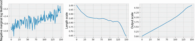
Inspect the jagged loss trajectory to see how numerical instability disrupts gradient-based optimization. section 12.1.3

How Bayesian Optimization in Action covers it

How deep it goes

Explains symptoms, optimization consequences, covariance failure, and automatic jitter, but does not derive numerical error bounds.

Examples

Uses jagged GP loss curves, non-positive-definite covariance warnings, large Sobol candidate sets, and automatic diagonal jitter.

What it assumes

Assumes familiarity with Gaussian processes, gradient descent, covariance matrices, and posterior sampling.

What you can do after

Diagnose unstable GP optimization from erratic losses and recognize covariance warnings repaired through automatic jitter.

How it connects

Connects Gaussian processes with gradient descent, marginal log likelihood, covariance matrices, jitter, and Thompson sampling.

liveBookmanning.com

Read Bayesian Optimization in Action on liveBook Get the book at manning.com

Related concepts

• jitteraddressed by · Jitter is a small perturbation added to values or model quantities to improve numerical stability, distinguish overlapping observations, or prevent repeated discrete outputs.
• determinantuses · A determinant is a scalar computed from a square matrix that characterizes properties such as invertibility and signed volume scaling.
• numerical stabilitycontrasts with · Numerical stability is the property of a computation that limits disproportionate error or loss of accuracy from small input perturbations and finite-precision arithmetic.

This explainer was generated by Manning's knowledge graph from the text of Bayesian Optimization in Action. The section links point to the parts of the book it draws on.