Linear time describes a running time that grows in proportion to the input being processed. The relevant input may be a list of goods, the characters in a string, cache entries, or another collection of elements. The bound describes how work scales, not whether the operation is fast in every practical setting. section 1.3.4 section 6.2.5
The input measure must be stated before interpreting a linear bound:
- For a greedy unbounded-knapsack algorithm, the work is linear in the already-sorted list of goods; sorting first changes the overall cost to linearithmic. section 1.3.4
- For a trie’s longest-prefix operation, the work is linear in the searched string’s length, written O(m) for a string of length m. section 6.2.5
- For Bloom-filter insertion, variable-length string keys make hashing linear in key length, while bounded-length keys can make the operation effectively constant with respect to stored elements. section 4.9.3
- For a simple LFU cache implementation, updating an entry can become linear in the number of cache elements when many counters tie and entries must be reordered. section 7.5.2
A cache update that becomes linear
Imagine a list of n cache entries whose frequency counters are equal. Accessing the entry at the end may require n−1 node swaps to move it toward the front. The operation is therefore linear in the number of entries for that edge case. Replacing the list with a priority queue changes the design and avoids this particular reordering pattern. section 7.5.2
Figure 7.10 An inefficient implementation of an LFU cache. When all elements of a list with n entries have the same value for counter, and one element at the end of the list is accessed, we will have to perform n-1 node swaps to bubble up the updated entry to the front of the list.
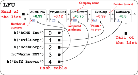
Shows how equal cache frequencies force an accessed entry through nearly the entire list, making the linear worst case visible. section 7.5.2