A partition divides a universe into groups that do not overlap and together contain its elements. For a food catalog, each item might belong to one group such as Fruit, Vegetables, or Sweets. The useful question is not just how to form the groups, but how to find an item’s group and update it efficiently. section 5.0 section 5.3
For dynamic groups, start with each element in its own singleton partition. Two operations do most of the work: areDisjoint(x, y) checks whether the elements belong to different partitions, and merge(x, y) combines their partitions. This is an aggregative model: groups can merge but cannot split. The relationship used to group elements must be reflexive, symmetric, and transitive. section 5.2 section 5.3
Grouping products
An online catalog can initially place every product in its own group, then merge products frequently bought together. The groups can support recommendations or let an algorithm work on each group instead of the entire catalog. New products and changing associations make efficient updates important. section 5.1
A direct implementation maps each element to a list representing its partition. Comparing list identities answers whether two elements share a group. Merging lists, however, requires updating the map entry for every element moved; that can take O(n) time for n elements. Appending the shorter list reduces the number of updates, but not the worst-case O(n) bound. section 5.4 section 5.4.1
A tree representation avoids updating every member on a merge. Each element points to its parent, and a root identifies its partition. To find an element’s partition, follow parent links to the root; to merge two partitions, link one root beneath the other. Root lookup determines the cost: it is logarithmic on average in this basic tree design, but can be linear if the tree degenerates into a chain. The representation stores a parent entry for each element. section 5.5.1 section 5.5.2
Figure 5.8 Merging two sets when using the tree representation. It only requires creating one new link (plus some tree traversing). In the figure on the left, we add one edge from the root tree of Tree 1 to the root of Tree 0, to merge them. On the right, we show how this changes the data structure: now we only have two trees, but the height of tree 0 is now larger than before the merge.
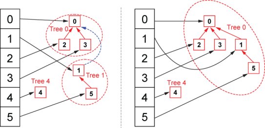
The diagram shows why a tree merge changes one parent link rather than every element’s partition entry—and why the resulting tree can grow taller. section 5.5.1
Partitioning a geometric space serves a different operation: locating points by region rather than repeatedly merging groups. A vertical line divides a plane into left and right regions, but ignores y coordinates and can put nearby points on opposite sides. Dividing a region into four quadrants uses both coordinates; a tree can assign one child to each quadrant. Points on dividing lines need a consistent assignment. In three dimensions, the corresponding split has eight octants, increasing the number of branches. section 8.4.2 section 8.4.3
Figure 8.10 Four-way partitioning of the plane. For each point, we split the area it belongs to in four quadrants using the lines passing through the point and parallel to the axes. For the first one, R in the example, we get four infinite quadrants (left). When we choose the next point, P (right), we have to further divide the upper-left quadrant into four parts: we get a finite rectangle, to which U belongs, and three infinite sections of the plane. For each further point, such as U, we further split the region it belongs to into four more smaller regions.
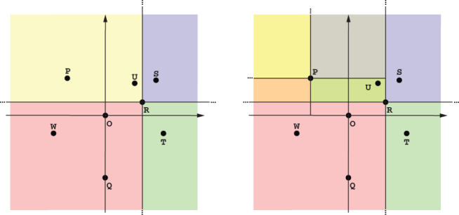
Successive points subdivide only the region containing them, making the four-way spatial partition concrete. section 8.4.3
