Pipeline efficiency measures the fraction of total pipeline execution time spent computing instead of waiting in idle bubbles. The 1F1B schedule improves it by interleaving forward and backward passes rather than completing all forwards first. section 6.5.4
For a pipeline with micro-batches and stages, efficiency is computed as: Number of Microbatches / (Number of Microbatches + Number of Stages - 1). section 6.5.4
Interpret the schedule in three phases:
- Warm-up fills the pipeline and creates an unavoidable initial bubble. section 6.5.4
- Steady state alternates forward and backward work to keep GPUs busy. section 6.5.4
- Cool-down drains the remaining gradients after forward work ends. section 6.5.4
Figure 6.7 The 1F1B interleaved schedule. Forward (blue) and backward (green) passes alternate during the steady state. Note: any small gaps visible in this rendered timeline are artifacts of the profiling resolution, not the schedule itself. In a true 1F1B, each GPU executes its remaining backward passes back-to-back during cool-down.
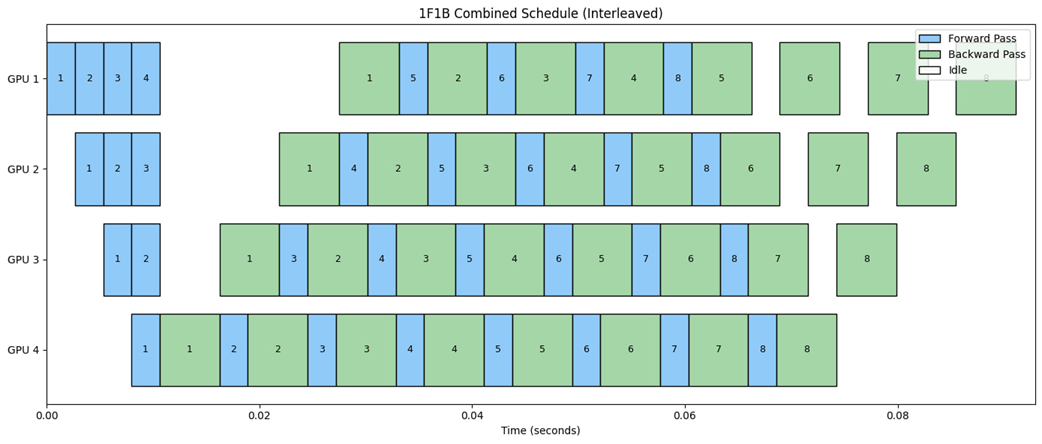
Use the schedule timeline to see forward and backward passes alternate densely during steady state, replacing large idle regions with computation. section 6.5.4
Efficiency = (Number of Micro batches) / (Number of Microbatches + Number of Stages - 1)
Use the equation to relate efficiency directly to the number of micro-batches and pipeline stages. section 6.5.4