Post-training quantization (PTQ) converts a trained model to lower precision by observing it on calibration data and deriving quantization parameters without gradient-based optimization. It is a fast, low-cost first choice: it can take minutes to hours and needs no training GPU cluster. section 4.0 section 4.1
Calibration data determines the activation ranges used to set scales and zero-points. If that data differs from production traffic, real inputs may exceed calibrated ranges, get clipped, and degrade answers. Use a few hundred representative samples, including edge cases and deployment scenarios, then validate accuracy against the FP32 baseline. section 4.0 section 4.5
Choose PTQ by weighing the factors that compound its accuracy risk:
- Consider architecture robustness, target bit-width, model size and redundancy, and the accuracy degradation the application can tolerate. section 4.1
- Expect PTQ to work best for INT8 CNNs and BERT-scale transformers with smooth weight distributions; INT4, small models, or strict accuracy budgets may require QAT. section 4.5 section 5.0
- Select a range estimator to fit the distribution: MSE performed best in reported experiments, while absmax suits clean distributions and percentile helps with sparse outliers. section 4.5
Calibration and measured accuracy
Calibrating a support chatbot on Wikipedia text can miss order IDs and code in customer tickets, causing clipping on production inputs. In reported INT8 experiments, MSE-optimal ranges produced 0.20% loss for ResNet and 0.00% for BERT. section 4.0 section 4.5
Figure 4.2 PTQ decision framework flowchart. Starting from the target bit-width at the top, the reader follows branching decisions through model architecture checks, calibration method selection, and accuracy validation gates. Each terminal node recommends either shipping the PTQ result or escalating to QAT.
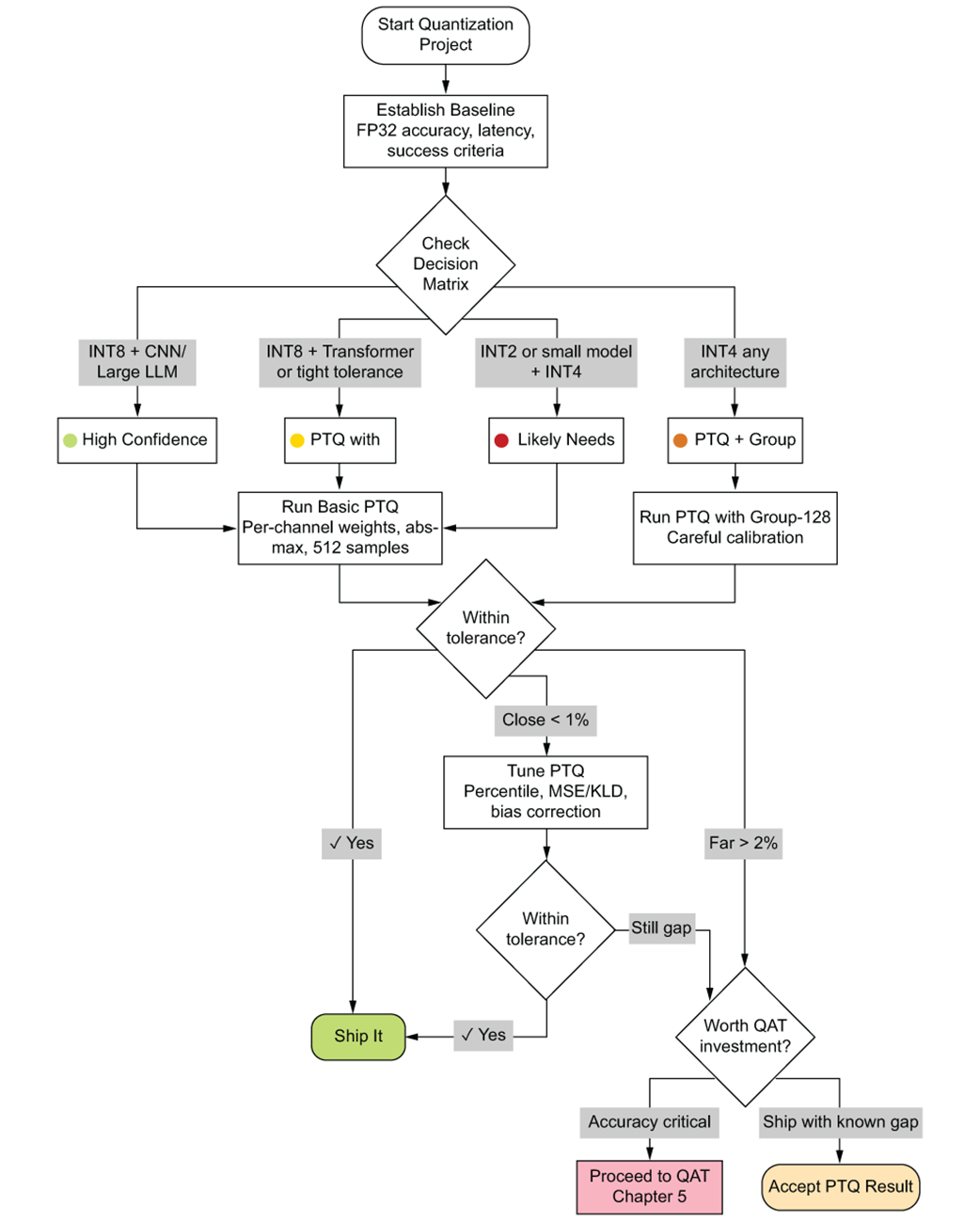
Use the decision flowchart to move from target bit-width through architecture, calibration, and accuracy checks to a PTQ or QAT recommendation. section 4.1
INT8 storage reduces model size by 4×, but latency improves only when the runtime supports quantized execution. PyTorch quantization backends, TensorRT, and ONNX Runtime are named options; storing INT8 weights alone does not speed inference. section 4.5