Pseudo-inverse

As explained in Math and Architectures of Deep Learning

A pseudoinverse is a generalized matrix inverse that provides least-squares solutions when an ordinary inverse does not exist.

A pseudo-inverse generalizes matrix inversion to nonsquare linear systems. It produces a solution that minimizes the error when an exact solution is unavailable, making it useful for overdetermined machine-learning models. section 2.12.4 section 2.12

For an overdetermined system A x ≈ b, transpose the system and solve the square normal equations. Assuming AᵀA is invertible, the resulting expression is A⁺ = (AᵀA)⁻¹Aᵀ. Unlike an ordinary inverse, this construction applies when A is not square. section 2.12.4

Geometrically, A x is the point in A’s column space closest to b. The residual b − A x is perpendicular to that column space, so the pseudo-inverse selects the least-squares projection. section 2.12.5

The pseudo-inverse connects linear algebra to model fitting in two complementary ways:

• Use augmented inputs to place model features and a bias term in one matrix X, then solve for weights with X⁺. section 2.12.5
• Use singular value decomposition to solve arbitrary systems without directly inverting A; for square invertible matrices, this agrees with the ordinary inverse solution. section 4.5.4

Fitting a toy threat-score model

Training examples pair hardness and sharpness with threat scores. After augmenting each input with 1 for the bias, the resulting overdetermined system estimates weights w₀, w₁, and b by minimizing the total prediction error. section 2.12.5 section 2.12

Figure 2.12 Solving a linear system A = is equivalent to finding the point on the column space of A that is closest to . This means we have to drop a perpendicular from to column space of A. If A represents the point where that perpendicular meets the column space (aka projection), the difference vector − A corresponds to the line joining and its projection A. This line will be perpendicular to all vectors in the column space of A. Equivalently, it is perpendicular to A for any arbitrary .

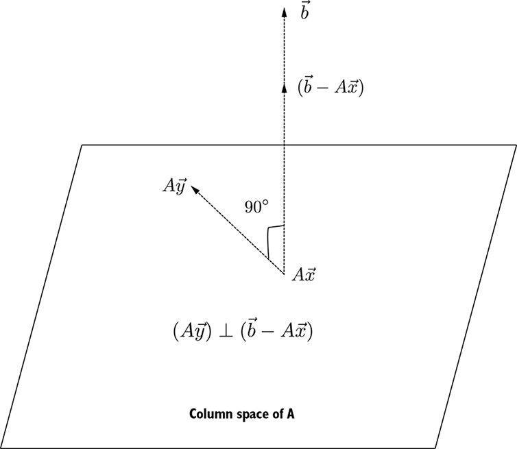
Inspect the geometric construction: projecting b onto the column space of A makes the residual perpendicular to every column-space direction. section 2.12.5

How Math and Architectures of Deep Learning covers it

How deep it goes

Defines the normal-equation formula, explains projection geometry, and derives an SVD route while deferring direct inverse computation.

Examples

Uses a toy cat-brain threat-score dataset, an augmented design matrix, projection geometry, and SVD-based system solving.

What it assumes

Assumes familiarity with matrix multiplication, transposes, linear systems, and column spaces while motivating the method through model fitting.

What you can do after

Apply it via matrix formulas or SVD to obtain best-fit solutions for nonsquare linear systems.

How it connects

Connects linear systems, least squares, matrix inverse, orthogonal projection, augmented matrices, and singular value decomposition.

liveBookmanning.com

Read Math and Architectures of Deep Learning on liveBook Get the book at manning.com

Also explained in

• 

  liveBookmanning.com
  Experimentation for EngineersA generalized matrix inverse that remains defined for some matrices whose ordinary inverse is undefined and agrees with the ordinary inverse when that inverse exists.

Compare how 2 books explain pseudo-inverse →

Related concepts

• matrix inverseequivalent to · A matrix inverse is a matrix that, when it exists, multiplies with a square matrix to produce the identity matrix.
• linear systemaddresses · A linear system is a set of linear relationships among variables, commonly expressed as simultaneous equations or a linear transformation, for which superposition applies.
• normal equationalternative to · A normal equation is a matrix equation whose solution provides the ordinary least-squares coefficients of a linear regression model.
• singular value decompositionproduced by · Singular value decomposition is a matrix factorization that expresses a matrix as the product of orthogonal or unitary matrices and a diagonal matrix of nonnegative singular values.
• transpositionuses · Transposition is an operation that exchanges a matrix’s rows and columns or, more generally, reorders the axes of a tensor without changing its values.
• PyTorchused by · PyTorch is an open-source machine-learning framework for Python that provides tensor computation, automatic differentiation, and tools for building and training neural networks.

This explainer was generated by Manning's knowledge graph from the text of Math and Architectures of Deep Learning. The section links point to the parts of the book it draws on.