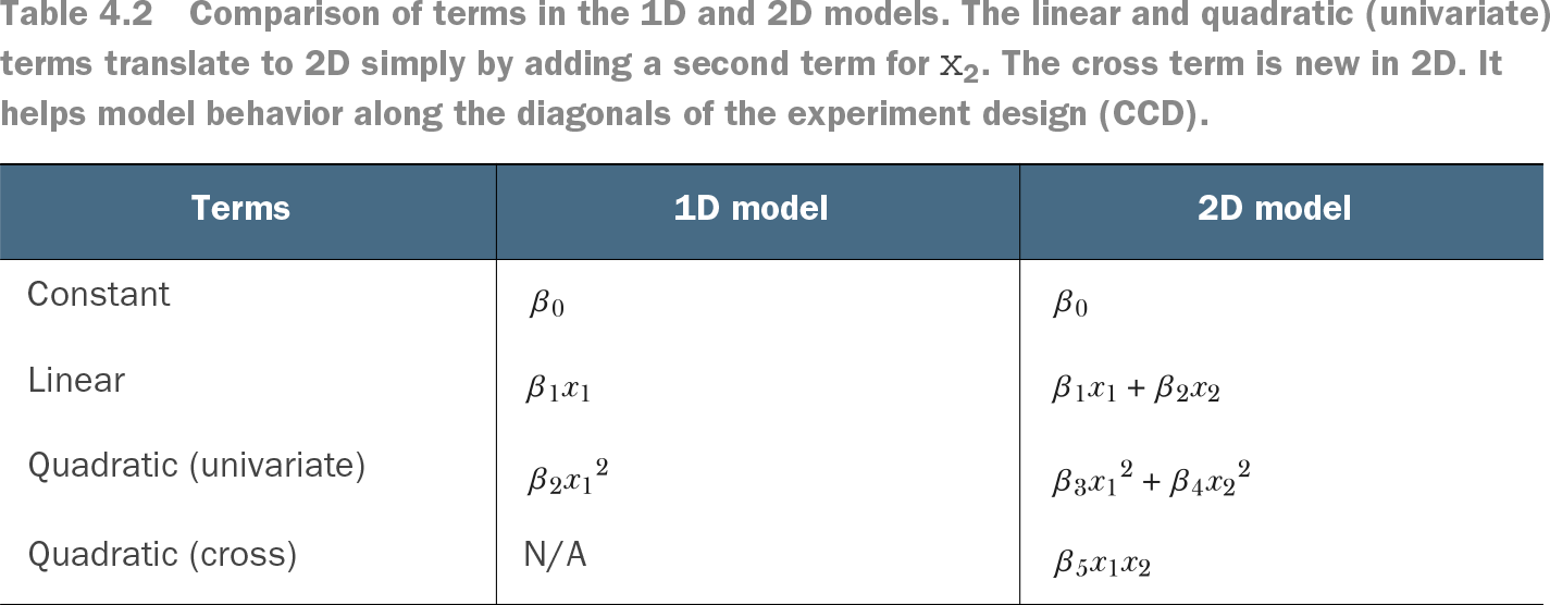
A quadratic model approximates a response surface with a constant, linear, squared, and pairwise-product term for each predictor. In two dimensions, the design matrix is [1, x₁, x₂, x₁², x₂², x₁x₂], allowing interpolation between measured parameter settings. section 4.2.2
Use the model within an iterative response-surface workflow:
- Measure the business metric at designed parameter settings and aggregate repeated observations with standard errors. section 4.2.2
- Fit the coefficients with linear regression, evaluate the fitted surface over a fine grid, and select its predicted maximum. section 4.2.2
- Shrink the parameter ranges around the current center when an extreme measurement suggests that the surface is too complex for the local model. section 4.2.2
- Validate the proposed optimum by measuring it directly; return to design if the result falls outside the estimate’s 95% confidence bounds. section 4.2.2
Trading-parameter search
For threshold and order_size, repeated experiments eventually produce a well-behaved local surface. The fitted model predicts threshold = 1.12 and order_size = 3.0, with estimated markout profit 0.41; a final experiment tests that estimate. section 4.2.2
Table 4.2 Comparison of terms in the 1D and 2D models. The linear and quadratic (univariate) terms translate to 2D simply by adding a second term for x2. The cross term is new in 2D. It helps model behavior along the diagonals of the experiment design (CCD). (view table figure)
Compare one- and two-predictor models to see why the cross term is needed for diagonal behavior in the experiment design. section 4.2.2