Quantization-aware training (QAT) adapts a model to deployment precision by simulating quantization during optimization. Try post-training quantization (PTQ) first: it avoids retraining and often suffices at INT8. Escalate when validation misses the accuracy target, especially at lower bit-widths, in small models, or under tight accuracy budgets. QAT can recover accuracy, but requires training compute, tuning, and engineering work. section 4.1 section 5.0
Fake quantization maps values to an integer grid, clips them to the supported range, then converts them back to floating point for the forward pass. Full-precision weights remain available for updates. Because rounding has zero gradient almost everywhere, a straight-through estimator (STE) substitutes a gradient of 1 through rounding. A clipped STE additionally zeros gradients for values outside the quantizable range. section 5.2 section 5.2.1
Rounding blocks the learning signal
With scale 0.5, quantize-dequantize maps inputs [0.3, 0.7, 1.2, 1.8] to [0.5, 0.5, 1.0, 2.0]. Backpropagating through ordinary rounding gives four zero gradients. An STE preserves the same simulated forward values while passing a surrogate gradient backward. section 5.2
Listing 5.4 Fake quantization with straight-through estimator
import torch
import torch.nn as nn

class FakeQuantizeSTE(torch.autograd.Function):
    """Fake quantization with straight-through estimator for gradients."""

    @staticmethod
    def forward(ctx, x, scale, zero_point, q_min, q_max):
        # Quantize: scale to integer range, round, clip
        x_int = torch.round(x / scale + zero_point)
        x_int = torch.clamp(x_int, q_min, q_max)

        # Dequantize: back to floating point
        x_q = (x_int - zero_point) * scale

        # Save for backward (needed for clipping gradient)
        ctx.save_for_backward(x, scale)
        ctx.q_min = q_min
        ctx.q_max = q_max
        ctx.zero_point = zero_point

        return x_q

    @staticmethod
    def backward(ctx, grad_output):
        x, scale = ctx.saved_tensors

        # STE: pass gradient through unchanged
        # But zero out gradients for values that were clipped
        x_int = x / scale + ctx.zero_point
        mask = (x_int >= ctx.q_min) & (x_int <= ctx.q_max)

        grad_input = grad_output * mask.float()

        # No gradient for scale, zero_point, q_min, q_max
        return grad_input, None, None, None, None

def fake_quantize(x, scale, zero_point, q_min, q_max):
    """Convenience wrapper for fake quantization."""
    return FakeQuantizeSTE.apply(x, scale, zero_point, q_min, q_max)
Inspect the fake-quantization forward pass and its STE-based backward pass. section 5.2
A practical QAT workflow:
- Validate PTQ against an FP32 baseline and profile layer sensitivity. Diffuse degradation may warrant QAT across layers; concentrated sensitivity can favor mixed precision instead. section 4.5 section 5.6
- Insert fake quantizers into selected convolutional or linear layers. A common configuration uses per-channel symmetric weights and per-tensor asymmetric activations; observers track ranges for quantization parameters. section 5.2.1
- Fine-tune with a lower learning rate, typically 1e-4 to 1e-5, for 5–20 epochs, with gradient clipping. Warm up the learning rate, freeze observer statistics after scales stabilize, and consider progressively lowering precision. section 5.2.2 section 5.6
- Monitor validation accuracy and scale changes together; stop when scales and accuracy have flattened. Verify that the deployment runtime supports the chosen precision and execution path: quantized storage alone does not guarantee faster inference. section 5.6 section 4.5
Per-channel weight quantization is especially useful when channel magnitudes vary widely: separate scales can prevent small channels from losing their gradients. Use output-channel axis 0 for convolutional and linear weights where the target supports it. The benefit is model-dependent: a small CNN with similarly sized channels showed nearly identical INT4 per-tensor and per-channel training curves. section 5.4.2 section 5.6
Selective transformer QAT
On BERT-base and SST-2, INT4 PTQ reached 50.9% accuracy. After three QAT epochs, attention-only quantization was within 0.11 percentage points of FP32, while quantizing all 72 linear layers was 1.61 points below it. Profile weight sensitivity before selecting layers; in this experiment, feed-forward layers dominated weight-quantization output error. Keep LayerNorm, softmax, and GELU in FP32. section 5.5 section 5.6
Figure 5.16 Selective QAT fine-tuning on SST-2 (INT4, 3 epochs). Left: accuracy per epoch. Right: best accuracy by strategy. QAT recovers BERT from the INT4 PTQ catastrophe (50.9%) to within 1.6% of FP32. Attention-only (48 layers at INT4) nearly matches FP32 at just −0.11%. FFN-only (24 layers) costs −0.57%. Quantizing all 72 layers incurs the largest gap (−1.61%).
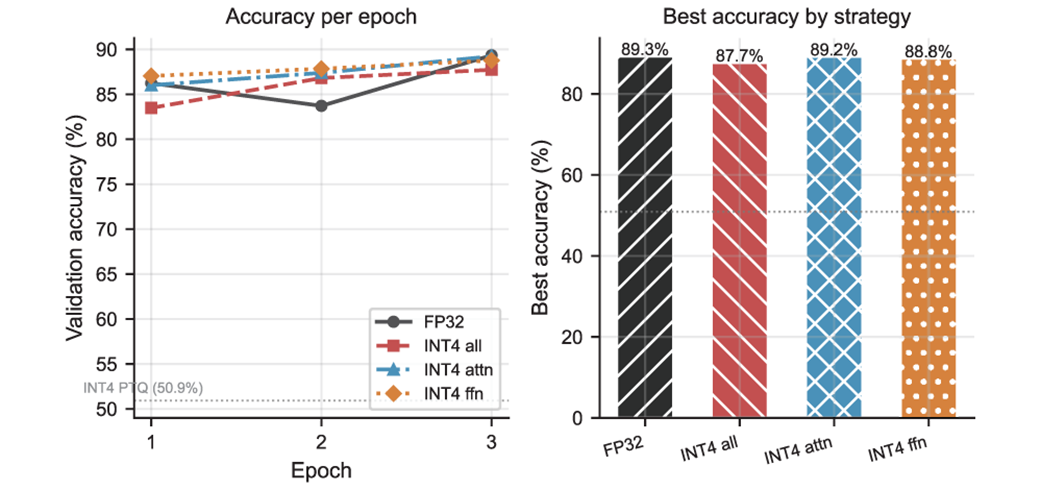
Compare accuracy across selective INT4 QAT strategies and the FP32 baseline. section 5.5
QAT is commonly used for fine-tuning, but can also train a model from scratch under a low-precision constraint. In a toy regression experiment with ternary weights, a BitLinear model trained with QAT reached test MSE 0.0070, versus 0.0199 for post-hoc ternarization of the FP32 model. section 5.2.2 section 8.5.2