Quantization calibration measures representative model values to choose the range and parameters of a quantization grid. It is especially important for activations, whose ranges depend on the input. Calibration data that differs from production traffic can produce excessive clipping or waste resolution. section 3.1 section 4.0
For a fixed number of integer levels, the range is a tradeoff. A wider grid clips fewer values but increases the step size and rounding error. A narrower grid gives typical values finer resolution but clips more outliers. For values inside a uniform grid, rounding error is bounded by half the step size; clipping error has no such bound. section 2.3
Figure 2.5 The granular-versus-overload error tradeoff. Widening the quantization grid (increasing the clipping range) reduces overload error—fewer values are clipped—but coarsens the step size, increasing granular error for values inside the range. Tightening the grid does the reverse. The optimal clipping boundary minimizes total distortion and depends on the shape of the data distribution: heavy-tailed distributions push the boundary outward; tightly concentrated distributions pull it inward.
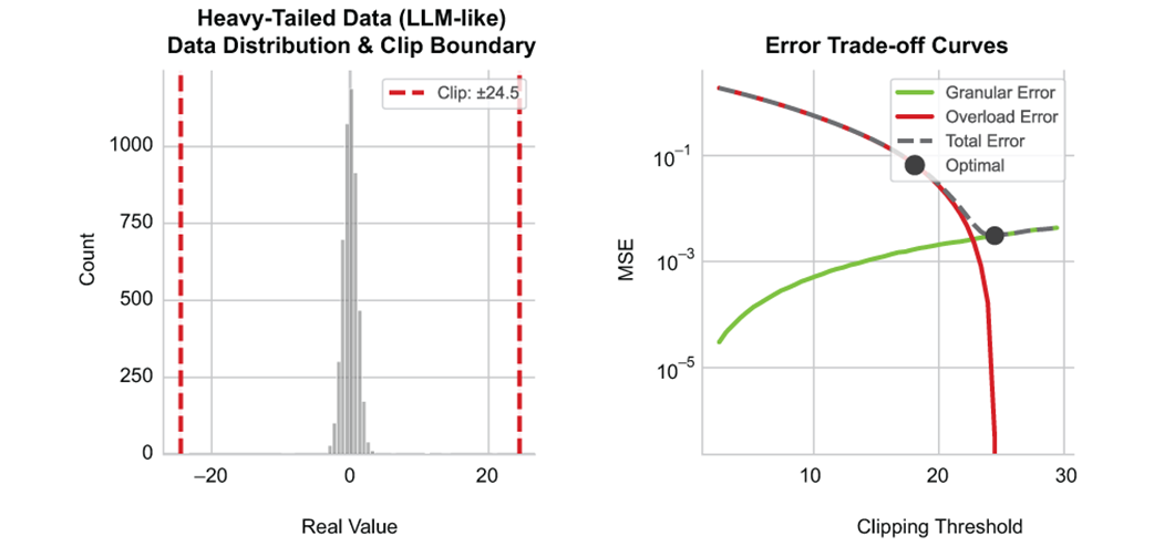
The figure shows how changing the clipping boundary trades rounding error against clipping error. section 2.3
A practical calibration workflow is:
- Run representative production-like inputs through the model and collect activation statistics across batches. Weight ranges can be measured directly; activation ranges depend on the inputs. section 3.1 section 2.6
- Choose range boundaries. Running minimum and maximum preserve observed extremes; percentile clipping can sacrifice outliers for finer resolution. Entropy minimization is another range-estimation option. section 3.1 section 2.6
- Derive scale and zero-point for the selected integer range. Validate the quantized model against a floating-point baseline and recalibrate if input distributions drift. section 2.5 section 2.6 section 4.0
For symmetric INT8 weights using integer codes [−127, 127], set the zero-point to 0 and the scale to the observed absolute maximum divided by 127. For affine activations, the scale spans the chosen real range over the integer range, and the zero-point shifts the grid. One implementation includes zero in the real range and handles a zero-width range separately. section 2.5
Listing 3.5 Calibration observer for activation ranges
class ActivationObserver:
    def __init__(self):
        self.min_val = float('inf')
        self.max_val = float('-inf')

    def observe(self, tensor):
        self.min_val = min(self.min_val, tensor.min().item())   #A
        self.max_val = max(self.max_val, tensor.max().item())

    def get_scale_zeropoint(self, bits=8, symmetric=False):
        if symmetric:
            abs_max = max(abs(self.min_val), abs(self.max_val))
            q_max = (1 << (bits - 1)) - 1
            scale = abs_max / q_max
            zero_point = 0
        else:
            q_min, q_max = 0, (1 << bits) - 1
            scale = (self.max_val - self.min_val) / (q_max - q_min)
            zero_point = int(round(q_min - self.min_val / scale))  #B
        return scale, zero_point
This observer accumulates activation minima and maxima across batches and derives symmetric or asymmetric parameters. section 3.1
Outliers and resolution
In one activation sample, absolute-max calibration gives a scale of 0.7222, while the 99th-percentile boundary gives 0.0115: the full-range grid is 63 times coarser. The percentile grid improves resolution for typical values but clips values beyond its boundary. section 3.1
Calibration supports post-training quantization without retraining or gradients. Check quality on production-like data, and match the integer representation to the target runtime and hardware: integer matrix multiplication requires both weights and activations quantized, with suitable hardware support. section 4.0 section 3.1