Rational Bézier curve

As explained in Geometry for Programmers

A rational Bézier curve is a Bézier curve defined using weighted basis functions normalized by their weighted sum.

A rational Bézier curve extends an ordinary Bézier curve by assigning each control point a weight. It evaluates weighted basis functions in the numerator, divides by their weighted sum, and gains extra control over the curve’s shape. section 7.2.3

The extra weights make the representation useful when ordinary polynomial Bézier curves are not precise enough:

• Changing a control point’s weight changes how strongly that point influences the curve, even when the control points remain fixed. section 7.2.3
• Rational Bézier curves represent conic sections such as circles, ellipses, and hyperbolas exactly. section 7.2.3 section 7.6
• The additional multiplications and division make them computationally heavier than polynomial Bézier curves. section 7.2.3
• CAD favors rational curves for precision, while 2D graphics and typography often prefer ordinary polynomial Bézier curves for speed. section 7.2.3

Adding weights to a cubic curve

For control coordinates xs = [0, 0.3, 0.7, 1], ys = [0.2, 0.8, 1, 0.5], and weights ws = [1, 2, 2, 1], compute the usual cubic basis terms twice: multiply each coordinate term by its corresponding weight for the numerator, multiply each basis term by that weight for the denominator, then return numerator / denominator. Keeping the control points fixed while trying weights such as (1, 1, 1, 1), (1, 2, 2, 1), or (1, 1, 4, 1) produces visibly different curves. section 7.2.3

Listing 7.10 Rational Bézier curve example

xs = [0, 0.3, 0.7, 1]                    #1
ys = [0.2, 0.8, 1., 0.5]                 #1
ws = [1., 2., 2., 1.]                    #1
 
def b3x(t, xs):                          #2
    n = ((1-t)*(1-t)*(1-t)*xs[0]*ws[0]   #2
        + 3*(1-t)*(1-t)*t*xs[1]*ws[1]    #2
        + 3*(1-t)*t*t*xs[2]*ws[2]        #2
        + t*t*t*xs[3]*ws[3])             #2
    d = ((1-t)*(1-t)*(1-t)*ws[0]         #2
        + 3*(1-t)*(1-t)*t*ws[1]          #2
        + 3*(1-t)*t*t*ws[2]              #2
        + t*t*t*ws[3])                   #2
    return n / d                         #2
def b3y(t, ys):
    return b3x(t, ys)

Use the listing to inspect the executable numerator-and-denominator calculation for a rational cubic Bézier curve. section 7.2.3

Figure 7.18 Cubic Bézier curves with the same control points with different weights, from left to right and top to bottom: (1, 1, 1, 1), (1, 2, 2, 1), (1, 0, 0, 1), (1, 1, 4, 1)

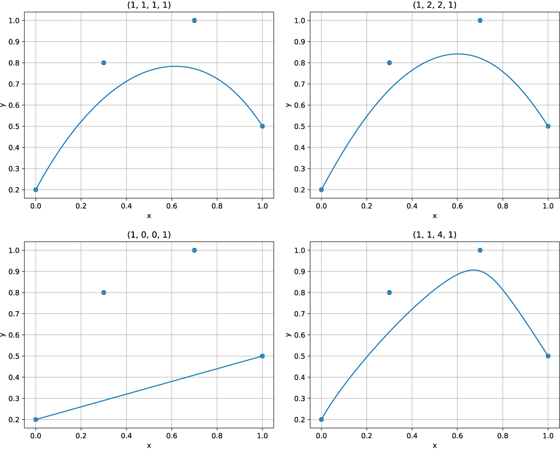
Compare how several weight sets reshape the same cubic control polygon. section 7.2.3

How Geometry for Programmers covers it

How deep it goes

Explains weighted normalization, provides a cubic implementation, compares shapes, and notes computational trade-offs.

Examples

Demonstrates a weighted cubic implementation and compares four weight sets applied to identical control points.

What it assumes

Assumes familiarity with Bézier curves, polynomial bases, control points, and basis functions.

What you can do after

Build it from scratch by evaluating weighted cubic basis terms and selecting weights for shape or precision.

How it connects

Connects Bézier curves, polynomial modeling, conic sections, splines, and NURBS.

liveBookmanning.com

Read Geometry for Programmers on liveBook Get the book at manning.com

Related concepts

• polynomial functionuses · A polynomial function is a function expressible as a finite sum of constant multiples of nonnegative integer powers of one or more variables.
• Bézier curvekind of · A Bézier curve is a parametric curve whose shape is determined by control points through Bernstein basis functions.
• splineimplements · A spline is a piecewise-polynomial function whose segments join at designated points with specified continuity or smoothness conditions.

This explainer was generated by Manning's knowledge graph from the text of Geometry for Programmers. The section links point to the parts of the book it draws on.