Reparameterization trick

As explained in Causal AI

A reparameterization trick rewrites a stochastic variable as a deterministic function of newly introduced exogenous random variables while preserving its marginal distribution.

A reparameterization trick rewrites a stochastic variable as a deterministic function of newly introduced exogenous random variables. The resulting structural causal model preserves the original observable distributions while making the generation mechanism explicit: sample noise, then assign values through functions. section 6.1.2 section 6.2.1

A practical conversion follows these steps:

• Introduce exogenous variables with distributions that contain the original uncertainty. section 6.1.2
• Define deterministic functions that map the exogenous variables and their parents to endogenous values. section 6.1.2
• Check that the observable marginal and conditional distributions remain unchanged. section 6.1.2
• Treat distributional equivalence as insufficient for causal equivalence: different mappings can imply different causal assumptions. section 6.2.1

Normal variables in a femur–height model

Sample n_x from Normal(0, 2.3) and n_y from Normal(0, 3.3), then assign x := 47 + n_x and y := 25 + 3x + n_y. Linear transformations preserve the original distributions for X and Y given X, but the model now exposes deterministic structural assignments. section 6.1.2

Bernoulli outcomes through stick breaking

For a coin with heads probability p_x, sample a uniform point between 0 and 1 and return heads when it falls within a region of length p_x. The same construction extends to multiple outcomes by partitioning the stick into probability-proportional regions. section 6.2.1

Listing 6.2 CGM rewritten as an SCM

from pyro.distributions import Normal
from pyro import sample

def scm_model():
    n_x = sample("n_x", Normal(0., 2.3))    #1
    n_y = sample("n_y", Normal(0., 3.3))   #1
    x = 47. + n_x     #2
    y = 25. + 3.*x + n_y    #2
    return x, y    #3

Compare the stochastic CGM with its deterministic-assignment SCM implementation. section 6.1.2

Figure 6.13 Two different ways of reparameterizing a causal generative model yield two different SCMs. They encode the same joint probability distribution but different endogenous values given the same exogenous value.

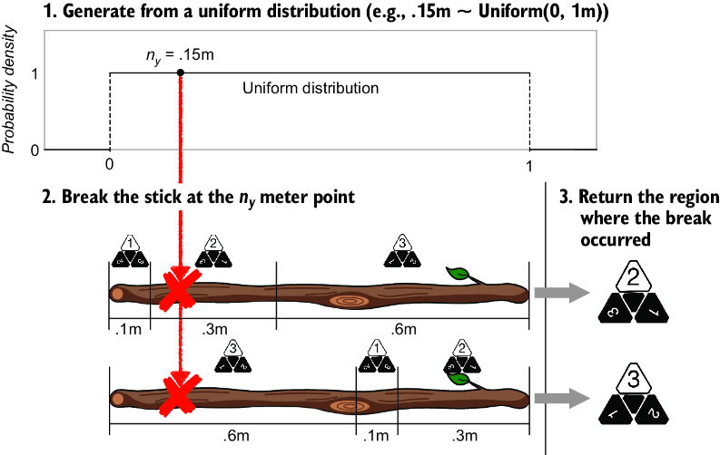
Inspect why two reparameterizations can preserve the joint distribution while assigning different endogenous values to the same exogenous value. section 6.2.1

How Causal AI covers it

How deep it goes

Explains normal and discrete constructions, then cautions that distributional preservation does not identify a unique causal model.

Examples

Uses a femur–height model, a weighted-coin flip, uniform stick breaking, and a three-sided die.

What it assumes

Assumes familiarity with probability distributions and causal graphs while introducing exogenous variables and deterministic structural assignments.

What you can do after

Evaluate alternative SCM constructions by checking distributional preservation and the causal assumptions induced by their mappings.

How it connects

Connects structural causal models, causal generative models, exogenous variables, deterministic functions, normal distributions, and Bernoulli distributions.

liveBookmanning.com

Read Causal AI on liveBook Get the book at manning.com

Related concepts

• variational autoencoderused by · A variational autoencoder is a generative neural network that learns a probabilistic latent representation of data and decodes samples from it to reconstruct or generate data.
• variational graph autoencoderused by · A variational graph autoencoder is a probabilistic graph autoencoder whose encoder defines a distribution over latent representations and whose decoder reconstructs graph-related inputs or structure.
• backpropagationaddresses · Backpropagation is a procedure for computing derivatives of an output or loss with respect to inputs and parameters by applying the chain rule backward through a computational graph.
• structural causal modelproduces · A structural causal model represents causal relationships among variables through equations that determine each variable from other variables and exogenous factors.
• samplingaddresses · Sampling is a procedure for selecting or generating observations, values, or outcomes from a larger population, signal, or probability distribution according to a specified method.
• timestepuses · A timestep is a discrete position or interval in an ordered temporal or sequential process at which state, computation, or output may change.

This explainer was generated by Manning's knowledge graph from the text of Causal AI. The section links point to the parts of the book it draws on.