ReZero

As explained in Inside Deep Learning: Math, Algorithms, Models

A training trick for residual-style networks that gates residual branches with a learnable scalar initialized to zero so the network starts near linear and gradually becomes more expressive.

ReZero adds a learnable gate α to each residual branch so a residual network starts as a simple linear path and gradually admits nonlinear depth. section 14.2 section 14.2.1

The residual branch is written as h = x + α⋅ReLU(F(x)), with α initialized to 0. At the start, the subnetworks are effectively off; during training, each α can grow independently and reintroduce its branch. section 14.2 section 14.2.1

Practical effects emphasized here include:

• faster early learning because the effective model is minimal at the start. section 14.2.1
• more flexible use of depth because each residual block can stay near zero or contribute more strongly. section 14.2.1
• fewer epochs to converge on deeper problems, especially with large models. section 14.0 section 14.5

PyTorch residual block switch

A residual block keeps F(⋅) in an nn.Sequential module and adds self.alpha as a learnable Parameter when the ReZero flag is enabled. A deeper CIFAR-10 residual network then compares ReZero=True against the standard residual version. section 14.2.2 section 14.2.2

Figure 14.3 Architecture of ReZero for two layers of a network. The shortcut path at the top allows easy gradient flow to the layers, and the long path at the bottom does all heavy work. Instead of simply adding back in the results of the subnetworks from the long path, we multiply them by α before adding them back in.

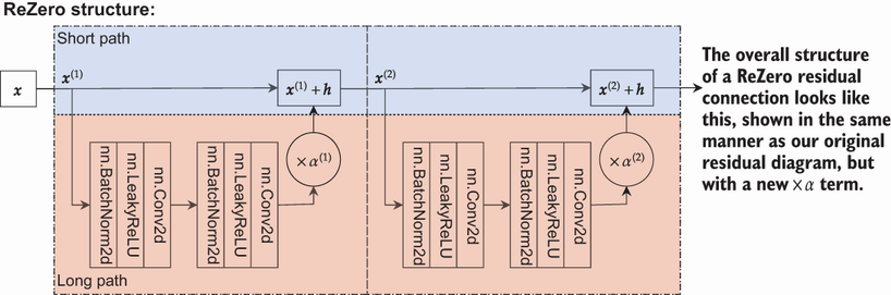
Shows the gated residual equation and the shortcut path that multiplies the branch by α before adding it back. section 14.2.1

Figure 14.4 ReZero’s behavior at the start of training for two layers of a network. The shortcut path at the top make a single linear layer (x⁽¹⁾ = x⁽²⁾) because nothing is added into them. The subnetworks in the long path are effectively gone because their contributions were multiplied by α = 0.

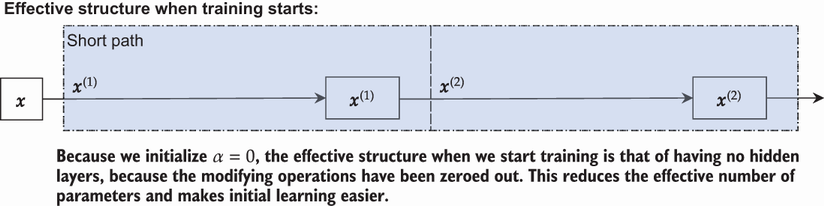
Shows the start-of-training behavior where α = 0 makes the residual branches disappear and leaves a linear architecture. section 14.2.1

Figure 14.5 ReZero architecture with several epochs of training. As the model trains, it can learn to change each α independently, slowly adding hidden layers back into the network. This way, it gradually learns to use the depth and select the total effective depth it desires based on the data. In this case, ReZero learned that it only needed one of its layers; for the second, it learned to keep α ≈ 0.

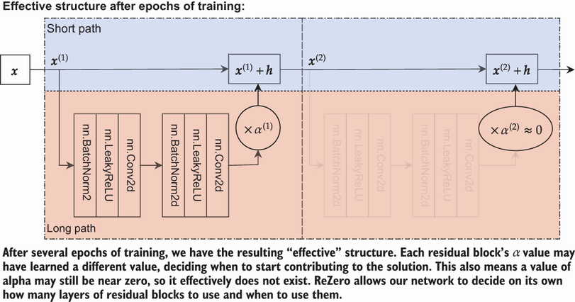
Shows training-time behavior where different α values recover depth at different rates and some branches may remain near zero. section 14.2.1

How Inside Deep Learning: Math, Algorithms, Models covers it

How deep it goes

Explains the residual equation, initialization, and training effect, then stops at implementation rather than theoretical proof.

Examples

Uses a CIFAR-10 residual network, plotted training curves, and a ResidualBlock code example with a ReZero flag.

What it assumes

Assumes residual-block basics and introduces the gate idea from zero.

What you can do after

Operate residual blocks that start linear, then learn to activate depth as training proceeds.

How it connects

Connects residual connections, skip connections, PyTorch, and residual blocks.

liveBookmanning.com

Read Inside Deep Learning: Math, Algorithms, Models on liveBook Get the book at manning.com

Related concepts

• parameteruses · A model parameter is a numerical value, such as a weight or bias, that is learned or set to determine how a model computes outputs.
• alphauses · A learned scalar coefficient that scales the residual branch in ReZero and is initialized to zero at the start of training.
• residual connectionimplements · A residual connection is a neural-network pathway that carries an earlier representation around one or more transformations to a later computation, where it can be combined with the transformed representation.
• convergenceproduces · Convergence is the process or property by which successive states or results approach a stable, limiting, or mutually consistent outcome.
• learning rate scheduleuses · A learning rate schedule is a rule or function that determines how an optimizer’s learning rate changes during training.

This explainer was generated by Manning's knowledge graph from the text of Inside Deep Learning: Math, Algorithms, Models. The section links point to the parts of the book it draws on.