A risk-free asset delivers a known return over the investor’s exact horizon. It is not merely a bond without credit risk: its maturity must match that horizon, and it must have no interim coupons that create reinvestment risk. A one-month Treasury bill held for a one-month horizon qualifies; a 10-year government bond sold after one month does not, because its sale price can create gains or losses. section 2.4
Because its return is certain over that horizon, the asset has zero volatility. On a mean–standard-deviation plot, it sits on the vertical axis at the risk-free rate. Combining it with a risky tangent portfolio creates feasible portfolios on the capital allocation line, which lies above the risky-asset efficient frontier. section 2.4
Use the risk-free asset to separate two portfolio decisions:
- Choose the risky portfolio, represented by the tangent portfolio on the capital allocation line. section 2.4
- Choose the allocation between that risky portfolio and the risk-free asset according to risk tolerance. For example, 70% in the tangent portfolio and 30% risk-free lies 70% of the way toward the tangent point. section 2.4 section 2.9
- Recognize that calling the line a capital market line additionally assumes the tangent portfolio is the market portfolio under shared information and expectations; capital allocation line avoids that assumption. section 2.4
For a target expected portfolio return μp, let Rf be the risk-free return, w0 its weight, w the risky-asset weights, μ expected risky returns, and Σ their covariance matrix. The constraints are μᵀw + Rf w0 = μp and 1ᵀw + w0 = 1. Eliminating w0 gives (μᵀ − Rf1ᵀ)w = μp − Rf, so the minimum-variance risky weights are proportional to Σ⁻¹(μ − Rf1). section 2.8
A horizon-matched holding
For a one-month objective, a one-month T-bill has a known payoff at the end of the month and therefore zero volatility in this model. Holding a 10-year government bond for that same month is different: even without credit risk, its resale price can vary before the horizon ends. section 2.4
The same zero-volatility case matters in goals-based dynamic programming. When an allocation is 100% risk-free bonds, the return-volatility input is zero; transition-probability calculations must handle division by zero rather than treat the outcome as a normal risky-return distribution. section 6.2.1
Figure 2.4 Risk–reward plot with a capital allocation line
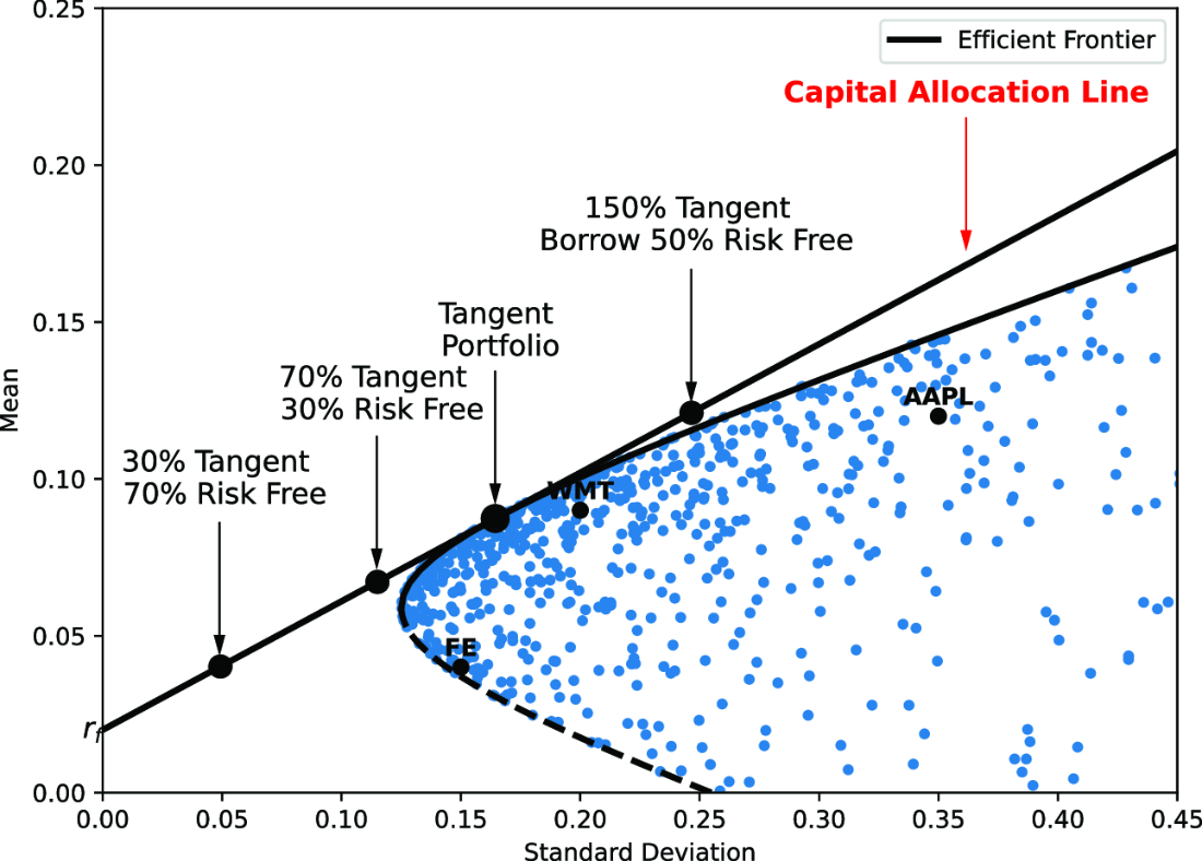
Inspect the plot to see the risk-free rate on the vertical axis and the straight capital allocation line connecting it to the tangent portfolio. section 2.4
