A shortest path connects two graph vertices with the least total distance or cost. In delivery routing, it identifies an efficient route from a warehouse to a customer while modeling intersections as vertices and streets as edges. section 14.0 section 14.3.1
A practical treatment develops the problem incrementally:
- Start with a regular city grid, where counting blocks approximates route length. section 14.3.1
- Represent intersections as vertices and one-way streets as directed edges; model two-way streets with paired edges. section 14.3.1
- Use breadth-first search when each traversed edge has equal cost, then reconstruct the route from the recorded distances and predecessors. section 14.3.6
- Recognize that weighted or differently optimized routes may require algorithms such as Dijkstra’s or A* rather than simple block counting. section 14.0 section 14.3.1
Delivery across a city grid
On a regular street grid, the shortest route between two intersections corresponds to minimum Manhattan distance: the sum of the absolute coordinate differences. Removing one connecting street can force BFS to select a completely different route. section 14.3.6
Figure 14.15 The shortest path to destination, and shortest distances to all the vertices, computed using BFS on the graph in figure 14.10. The shortest path is shown with dashed arrows, while distances are shown next to each vertex.
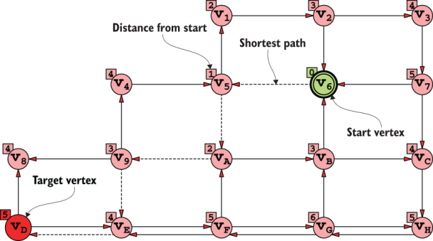
Use the diagram to inspect BFS-computed distances for every vertex and trace the selected path to the destination. section 14.3.6