Stationary distribution

As explained in Machine Learning Algorithms in Depth

A stationary distribution is a probability distribution that remains unchanged under the transition dynamics of a stochastic process.

A stationary distribution describes how probability is spread across the states of a Markov chain after a transition leaves that distribution unchanged. It also represents the long-run frequency of visits when the chain settles into such behavior. A time-invariant chain has transition probabilities that do not change over time; that is a property of the transitions, not the definition of a stationary distribution. section 7.1

Let A be a transition matrix whose rows sum to 1, and let π₀ be an initial row vector of state probabilities. After n transitions, the distribution is π₀Aⁿ. A stationary distribution π satisfies πA = π, with entries that sum to 1. Thus π is a left eigenvector of A with eigenvalue 1. Repeated transitions provide a way to approach it when the chain's behavior permits convergence. section 7.1

Figure 7.1 A two-state Markov model

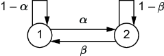
The two-state model makes each transition probability—and the requirement that probabilities leaving a state sum to 1—visible. section 7.1

Ranking web pages

Represent pages as states and links as possible transitions. The stationary probability πⱼ serves as page j's rank. Following links alone can leave pages unreachable or produce oscillation, so the transition rule also allows a uniformly chosen page; pages with no outgoing links use that random jump. For a large transition matrix, an iterative power method seeks the relevant eigenvector rather than treating ranking as a separate scoring rule. section 7.1.1

The same idea gives Markov chain Monte Carlo its target: construct a chain whose stationary distribution is the posterior p(θ|x). A random walk through parameter space then spends time in states in proportion to that posterior, supplying samples for Monte Carlo estimates. section 2.0 section 1.4.1

How Machine Learning Algorithms in Depth covers it

How deep it goes

Derives the fixed-point and eigenvector characterization, then applies iterative computation; leaves a stated existence proof as an exercise.

Examples

Uses a two-state Markov model and a web-link graph with random jumps to make transitions and long-run ranking concrete.

What it assumes

Assumes basic probability and matrix operations while introducing state transitions and their long-run distribution through a two-state model.

What you can do after

Build it from scratch: formulate a transition matrix and seek its stationary eigenvector using iteration for page ranking.

How it connects

Links Markov chains, transition matrices, eigenvectors, PageRank, Markov chain Monte Carlo, and posterior distributions.

liveBookmanning.com

Read Machine Learning Algorithms in Depth on liveBook Get the book at manning.com

Related concepts

• posterior probabilityequivalent to · A posterior probability or distribution expresses the probability assigned to an event, hypothesis, or unknown quantity conditional on observed evidence and prior information.
• PageRankequivalent to · PageRank is a link-analysis algorithm that estimates the relative importance of nodes in a directed graph from the structure and importance of incoming links.
• convergenceused by · Convergence is the process or property by which successive states or results approach a stable, limiting, or mutually consistent outcome.
• markov chain monte carloproduced by · Markov chain Monte Carlo is a family of sampling algorithms that generate samples using a Markov chain whose stationary or limiting distribution is a target probability distribution.
• eigenvectorequivalent to · An eigenvector is a nonzero vector that a linear transformation maps to a scalar multiple of itself.
• target distributionequivalent to · A target distribution is the probability distribution that a sampling procedure is intended to reproduce.

This explainer was generated by Manning's knowledge graph from the text of Machine Learning Algorithms in Depth. The section links point to the parts of the book it draws on.