A tensor operation takes numeric tensors—such as vectors or matrices—and produces tensor values. Adding, multiplying, and transforming tensors are the small steps from which neural-network layers are built. A familiar example is a dense layer: it transforms an input matrix into a new representation. section 2.3
dense <- function(inputs, W, b) {
  torch$nn$relu(torch$matmul(inputs, W) + b)
}
This PyTorch function shows a dense layer as three operations in sequence: multiply the inputs by weights, add a bias, then apply relu. section 3.4.1
Read the dense-layer expression from the inside out:
- matmul(inputs, W) combines the input tensor with the weight matrix W. section 2.3
- Adding b incorporates a bias vector into the result. section 2.3
- relu keeps positive values and replaces negative values with zero: relu(x) is max(x, 0). section 2.3
Tensor operations also have a geometric interpretation. Adding a vector moves a point; applying the same addition to many points translates an object without distorting it. A matrix product can rotate or scale points. Chaining operations lets a neural network make a much more complex transformation through simple steps. section 2.3.5 section 2.3.6
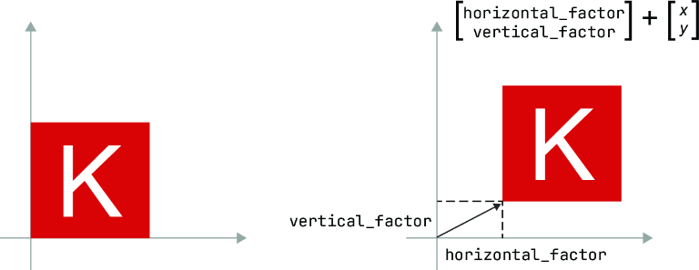
The figure makes vector addition concrete: every point of a 2D object moves by the same amount and in the same direction. section 2.3.5
During training, differentiable tensor operations have another useful property: gradients describe how changing tensor-valued weights changes the loss. Backpropagation combines gradients through the chain of operations, making it possible to update the weights. Frameworks such as PyTorch provide tensor operations and gradient computation; Keras provides higher-level layers and training tools. section 2.4.2 section 2.6 section 3.2


