Imagine searching a list of numbers. If the number is first, you find it immediately. If it is absent, you check every entry. Time complexity describes how the work an algorithm does grows as its input grows. It helps you compare approaches before implementing them, especially when large inputs or tight constraints make slow solutions impractical. section 1.3 section 1.3.1
Let N be the number of entries. Common growth patterns include:
- O(1), constant: accessing an array entry by index takes the same kind of operation as N changes. section 1.3.1
- O(log N), logarithmic: growth is much slower than a one-by-one scan; binary search is a search example. section 1.3.1
- O(N), linear: a linear search may compare against every entry, so more entries mean more checks. section 1.3.1
- O(N²), quadratic: the work grows with N × N, making increases in input size more costly. section 1.3.1
Figure 1.2 A graph showing the time complexities with varying inputs. O(1) is the constant time, while O(n!) shows the worst time. O(log n) is logarithmic, and O(n) is linear time. Quadratic and cubic are in between and work well for smaller values of n.
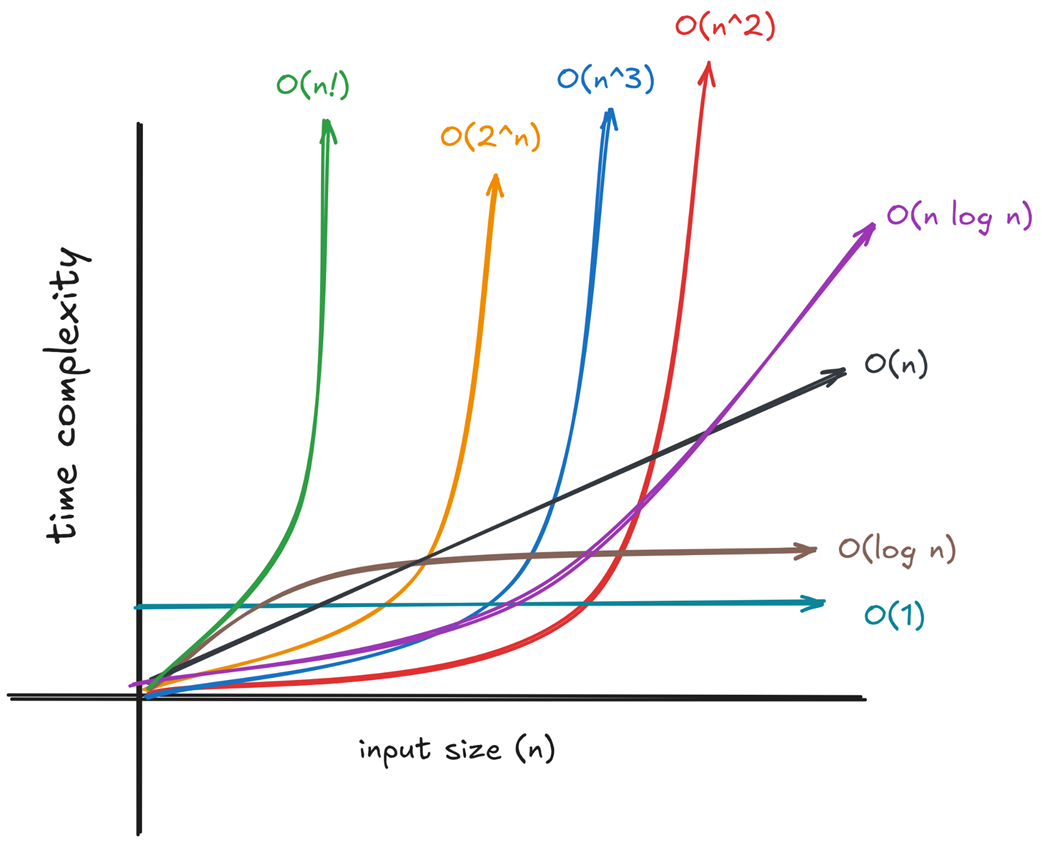
Compare the curves as input size increases: the useful question is not just which approach is quick on a small input, but how sharply its work grows. section 1.3.1
Which case should you report? For linear search, finding the first entry is the best case; an absent entry forces a full scan and gives the worst case. Best, average, and worst cases describe different conditions. Worst-case analysis is often useful when an edge case could hurt a larger system. section 1.3 section 1.5
The input measure matters
A two-dimensional knapsack calculation takes O(n × W) time, where n is the number of items and W is the capacity. Four items and a capacity of 8 produce a small table; keeping four items but raising the capacity to 800,000,000 makes the table and its loops enormous. A complexity label is only useful when you know what its variables measure. section 7.3
Time is not the only constraint. Breadth-first and depth-first graph traversals take O(V + E) time, where V counts vertices and E counts edges; they also use memory for a visited set. In string search, Rabin–Karp averages O(n + m), but repeated hash collisions can raise its worst-case time to O(n × m). Compare both the expected input and the difficult cases before choosing an algorithm. section 1.4.5 section 4.0