Variational free energy is an objective for approximating an intractable posterior distribution. Minimizing it is equivalent to maximizing a variational lower bound on model evidence. section 3.1 section 3.2
Let p̃(x) denote an unnormalized distribution and q(x) an approximating distribution. The objective combines an entropy-encouraging regularizer with expected energy, so q both remains broad and explains the data. Its optimum equals the log partition function when q matches the true posterior. section 3.1
The optimization has several linked interpretations:
- Minimizing variational free energy minimizes reverse KL divergence between q and the target posterior. section 3.1
- Maximizing the ELBO provides the equivalent lower-bound formulation derived using Jensen’s inequality. section 3.1
- Under a mean-field approximation, q factorizes into marginal distributions and each marginal is optimized while the others remain fixed. section 3.2
- The optimal marginal follows a distribution formed from the expected contribution of the remaining variables; its functional form depends on the variable type and probability model. section 3.2
Gaussian and mixture approximations
For p(x) distributed as N(0,1) and q(x) distributed as N(μ,4), the KL objective is smallest at μ = 0. For a four-component Gaussian mixture, forward KL spreads q across the support, whereas reverse KL concentrates q around one mode. section 3.1 section 3.1
Figure 3.1 KL(q||p) for p(x)∼N(0,1) and q(x)∼N(μ,4)
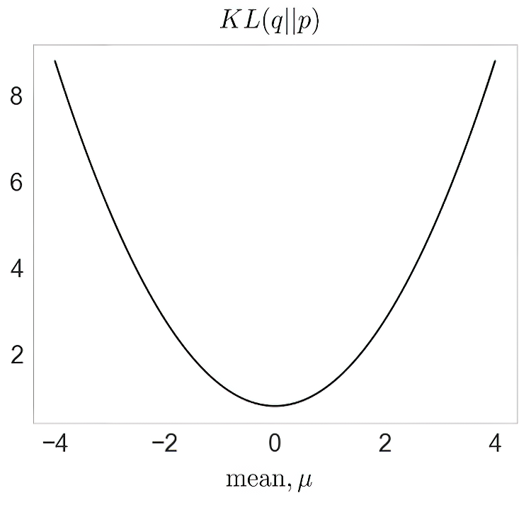
Visualizes the Gaussian KL objective as the approximating mean changes. section 3.1
Figure 3.2 Forward KL (left) q(x) overestimates the support, while reverse KL (right) q(x) locks onto a mode.
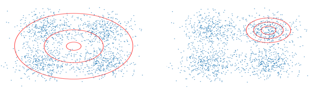
Contrasts forward-KL support spreading with reverse-KL mode seeking. section 3.1
Figure 3.3 True posterior (left), structured approximation (middle), and fully factored approximation (right)
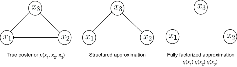
Compares a true posterior with structured and fully factored approximations. section 3.2
