Variational Gaussian process

As explained in Bayesian Optimization in Action

A variational Gaussian process is a scalable approximation to a Gaussian process whose posterior is represented through variational inference over a finite set of inducing points.

A variational Gaussian process (VGP) makes Gaussian-process regression practical when a full GP is too expensive to train on a large dataset. Instead of conditioning on every observation, it learns a small set of inducing points that represent the dominant trends in the data. The goal is predictions close to those of a GP trained on all data, with far less computation. section 12.0 section 12.5

The approximation is chosen by comparing two posterior distributions: one induced by the selected points and one associated with the full dataset. KL divergence measures their difference. Because directly optimizing that difference is impractical, training optimizes the evidence lower bound (ELBO), a computable proxy that lower-bounds marginal log likelihood. section 12.2.1 section 12.5

A VGP training workflow is:

• Choose an initial, relatively small set of inducing points rather than using the entire dataset directly. section 12.2 section 12.2.3
• Define a variational distribution over those points and a variational strategy for producing predictions from it. section 12.2.3
• Learn inducing-point locations and other model parameters by minimizing negative ELBO with mini-batch gradient descent. section 12.2.3 section 12.5
• Optionally use natural gradient descent for variational parameters while mini-batch gradient descent updates parameters such as length and output scales. section 12.5

Housing-price regression at scale

For California housing prices, a VGP can use the same mean and covariance functions as a regular GP while avoiding its prohibitive large-data training cost. Features include housing attributes, the target is normalized log median house value, and a Matérn 5/2 kernel with ARD models the inputs. Comparing training times exposes the efficiency gain. section 12.4 section 12.1.3

Figure 12.1 Predictions made by a regular GP and those by a VGP. The VGP produces almost identical predictions as the GP, while taking significantly less time to train.

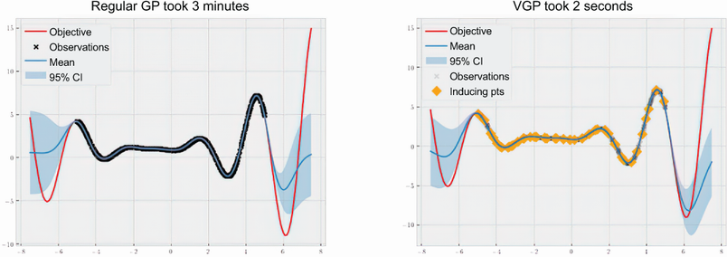
Compare the near-matching predictive behavior of a VGP and a regular GP against the VGP's substantially shorter training time. section 12.0

How Bayesian Optimization in Action covers it

How deep it goes

Develops inducing-point selection, KL divergence, ELBO training, mini-batches, and natural gradients, with a GPyTorch implementation.

Examples

Uses representative weather measurements, GP-versus-VGP prediction plots, and California housing-price regression.

What it assumes

Builds on regular GP training, mean and covariance functions, likelihoods, and gradient descent before introducing VGP-specific components.

What you can do after

Apply it via GPyTorch by defining variational components, learning inducing locations, and training with a mini-batch ELBO.

How it connects

Connects Gaussian processes with inducing points, KL divergence, ELBO, mini-batch gradient descent, natural gradient descent, and marginal log likelihood.

liveBookmanning.com

Read Bayesian Optimization in Action on liveBook Get the book at manning.com

Related concepts

• inducing pointuses · An inducing point is a selected input location whose associated function values summarize information from a larger dataset for a sparse Gaussian process approximation.
• Kullback–Leibler divergenceuses · Kullback–Leibler divergence is a nonnegative, directed measure of the information lost when one probability distribution approximates another, computed as an expected log ratio under the first distribution.
• variational strategypart of · A variational strategy is a GPyTorch abstraction that manages the variational approximation and its relationship to a Gaussian process model.
• approximate distributionpart of · An approximate posterior distribution is a tractable probability distribution selected or optimized to represent an intractable posterior distribution over unknown quantities.
• Gaussian processkind of · A Gaussian process is a probability distribution over functions in which every finite collection of function values has a joint Gaussian distribution.
• natural gradient descentused by · Natural gradient descent is an optimization method that updates parameters using gradients adjusted to the geometry of a model’s probability distribution.

This explainer was generated by Manning's knowledge graph from the text of Bayesian Optimization in Action. The section links point to the parts of the book it draws on.