Asymmetric quantization shifts an integer grid to fit a tensor’s range rather than centering it on zero. It can use more of the available codes for one-sided activations, but the zero-point shift introduces correction terms in inference arithmetic. section 2.4 section 2.6
The affine mapping reconstructs a real value as r ≈ S(q − Z), where S is the scale and Z is the integer coordinate for real zero. Quantization uses q = round(r/S) + Z, with results clamped to the integer range. Calibration sets S from the real and integer ranges and calculates Z from the minimum; the calibrated real range is extended to include zero. This preserves exact zero for uses such as ReLU sparsity and zero-padding. section 2.5 section 2.6
Mapping a shifted range
For a real range of [−1, 4] and integer range [0, 255], S = 5/255 ≈ 0.0196 and Z = 51. A real value of 1 maps to q = round(1/S) + 51 = 102; reconstruction gives S(102 − 51) = 1. Values between grid points are rounded, while values outside the calibrated range are clipped. section 2.5 section 2.6
Figure 2.6 Symmetric versus asymmetric quantization. Asymmetric quantization (left) shifts the grid to cover only the region the data actually occupies, reclaiming bits that would otherwise encode empty space. The zero-point Z records the shift, and must be accounted for during inference arithmetic. Symmetric quantization (right) pins the grid at zero and mirrors the range, making it ideal for centered distributions like weight tensors but wasteful for one-sided data.
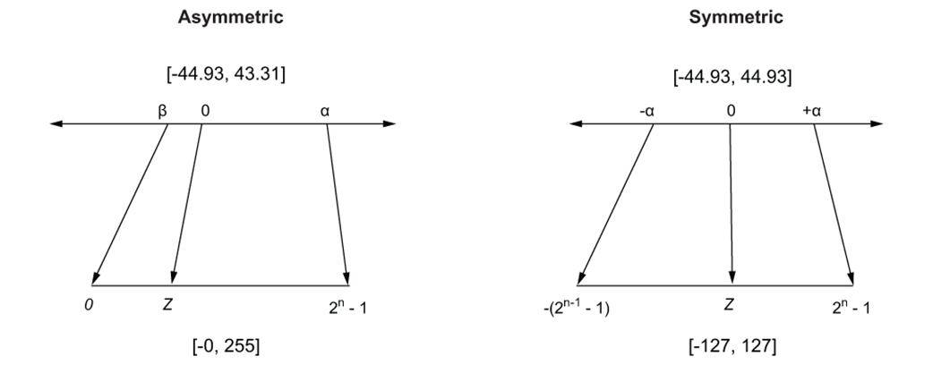
Compare a shifted grid with a zero-centered grid and see where the zero-point enters the tradeoff. section 2.4
The benefit depends on the distribution. For roughly zero-centered weights, a symmetric grid usually fits well and avoids offset arithmetic. ReLU activations are non-negative, so a symmetric grid reserves negative codes for empty space. An asymmetric activation grid can use the full integer range instead. section 2.4
Resolution on ReLU activations
In one comparison, symmetric quantization uses codes [0, 127] with scale 0.139, while asymmetric quantization uses [0, 255] with scale 0.069. The finer asymmetric grid provides approximately 2.01 times the resolution for that example. section 2.5
For a dot product, the integer terms expand as Σ(qx − Zx)(qw − Zw) = Σqxqw − ZwΣqx − ZxΣqw + nZxZw. Setting the weight zero-point Zw to zero removes the input-sum and constant terms. The remaining result is scaled by SxSw; the activation correction ZxΣqw must still be accounted for when Zx is nonzero. section 2.4 section 2.5
A correction that matters
For shifted activations with Zx = 48, a hybrid linear-layer experiment reports mean absolute error against FP32 of 0.0302 with correction and 1.4174 without it: a 46.9-fold increase in this case. section 2.5
Listing 2.9 Linear8bit layer with hybrid quantization
class Linear8bit(nn.Module):
    def __init__(self, in_features, out_features, bias=True):
        super().__init__()
        self.weight = nn.Parameter(torch.randn(out_features, in_features))
        self.bias = nn.Parameter(torch.randn(out_features)) if bias else None
        self.weight_quantizer = SymmetricQuantizer(bits=8)         #A
        self.input_quantizer = AffineQuantizer(bits=8)             #A

    def forward(self, x):
        self.input_quantizer.calibrate(x)
        x_q = self.input_quantizer.quantize(x)                     #B

        self.weight_quantizer.calibrate(self.weight)
        w_q = self.weight_quantizer.quantize(self.weight)          #C

        term1 = torch.mm(x_q.float(), w_q.float().t())             #D
        sum_w_q = torch.sum(w_q.float(), dim=1)
        term2 = self.input_quantizer.zero_point * sum_w_q          #E

        y_int = term1 - term2                                      #F
        scale = self.weight_quantizer.scale * self.input_quantizer.scale
        y_out = y_int * scale

        if self.bias is not None:
            y_out += self.bias
        return y_out
Inspect the hybrid linear layer’s separate weight and activation quantizers and its zero-point correction. section 2.5
A practical default is symmetric weights and asymmetric activations, provided the runtime supports the required correction efficiently. Calibration remains a tradeoff: a wider range reduces clipping but increases rounding error. Activation ranges can change between batches, so robust boundaries or recalibration may be needed when distributions drift. section 2.4 section 2.6