Bilinear Transformation
Definition
A bilinear transformation is a powerful mathematical tool used in geometry to transform shapes while preserving certain properties. Specifically, it can transform a square into a curvy concave object while maintaining straight lines. This transformation is more potent than a projective transformation and generalizes rotation, translation, and scale, which are all affine transformations. However, unlike affine transformations, bilinear transformations do not correspond to matrix multiplication.
In two-dimensional space, a bilinear transformation is characterized by each coordinate having its own formula, which is a product of two linear polynomials. This makes it a polynomial of two variables and allows it to be governed by four points, thus making it a four-point transformation.
Characteristics
- Non-linear Nature: Despite its name, a bilinear transformation is not linear. It is more versatile than a projective transformation, allowing for more complex shape manipulations.
- Dimensionality: While it generalizes well in 2D, it does not extend to 3D as smoothly as projective transformations. In 3D, a bilinear transformation becomes an eight-point transformation, compared to the (n+2)-point transformation of projective transformations in n-dimensional space.
Visual Examples
Transformation of a Square
A bilinear transformation can take a standard square and morph it into a curvy concave shape, as illustrated in the figures below:
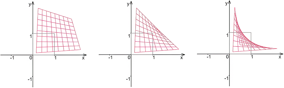 Figure 4.15 A bilinear transformation makes a square into a curvy concave object.
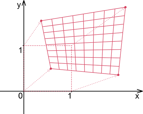 Figure 8.1 An example of a bilinear transformation of the standard square
Implementation
The following listing provides a straightforward approach to implementing a bilinear transformation. It involves solving a system of equations to determine the transformation parameters:
Listing 8.1 A straightforward approach for the bilinear transformation
a11, a12, a13, a14 = symbols('a11 a12 a13 a14')                  #1
a21, a22, a23, a24 = symbols('a21 a22 a23 a24')                  #1
x1, x2, x3, x4 = symbols('x1 x2 x3 x4')                          #1
y1, y2, y3, y4 = symbols('y1 y2 y3 y4')                          #1
xt1, xt2, xt3, xt4 = symbols('xt1 xt2 xt3 xt4')                  #1
yt1, yt2, yt3, yt4 = symbols('yt1 yt2 yt3 yt4')                  #1

system = [                                                       #2
    a11*x1*y1 + a12*x1 + a13*y1 + a14 - xt1,                     #2
    a21*x1*y1 + a22*x1 + a23*y1 + a24 - yt1,                     #2
    a11*x2*y2 + a12*x2 + a13*y2 + a14 - xt2,                     #2
    a21*x2*y2 + a22*x2 + a23*y2 + a24 - yt2,                     #2
    a11*x3*y3 + a12*x3 + a13*y3 + a14 - xt3,                     #2
    a21*x3*y3 + a22*x3 + a23*y3 + a24 - yt3,                     #2
    a11*x4*y4 + a12*x4 + a13*y4 + a14 - xt4,                     #2
    a21*x4*y4 + a22*x4 + a23*y4 + a24 - yt4                      #2
]

all_as = solve(system, (a11, a12, a13, a14, a21, a22, a23, a24)) #3
#1 The symbols are more or less like those in the formula, except that the initial positions of points lose the i index for brevity.
#2 The system consists of four pairs of “x transforms to xt” and “y transforms to yt” equations.
#3 On my computer, the solver works for about a quarter of a second.
This code snippet demonstrates how to set up and solve the equations necessary for performing a bilinear transformation, highlighting the complexity and power of this transformation technique.
FAQ (Frequently asked questions)
What effect does a bilinear transformation have on a square?
What is a bilinear transformation in 2D?
How many points govern a bilinear transformation?
What does Figure 8.1 show about bilinear transformations?
What is a bilinear transformation?
How does a bilinear transformation differ from matrix multiplication?
What does Figure 4.15 illustrate about bilinear transformations?
What is Listing 8.1 about in the context of bilinear transformations?
How are the transformation parameters solved in Listing 8.1?