Latent Semantic Analysis (LSA)
Overview
Latent Semantic Analysis (LSA) is a powerful technique used in natural language processing to identify and group semantically similar terms into topics based on their co-occurrence in documents. Unlike traditional methods that rely on cosine similarity for measuring document similarity, LSA captures latent semantic similarities by identifying shared topics rather than exact word matches. This is achieved through the use of Singular Value Decomposition (SVD), which finds principal components that represent topics as directions in the document feature space.
Definition
LSA is a technique for topic modeling that involves performing Principal Component Analysis (PCA) on document vectors to identify topics. This allows LSA to detect latent similarities beyond direct term overlap, making it a robust method for understanding the underlying semantic structure of a collection of documents.
Computing LSA
The process of computing LSA involves several steps, as demonstrated in the following code listing:
Listing 4.8 Computing LSA
terms = ["violence", "gun", "america", "roses"]         #1
X = torch.tensor([[0, 0, 0, 2],
              [1, 1, 1, 0],
              [2, 2, 0, 0],
              [3, 3, 0, 0],
              [5, 5, 0, 0],
              [0, 1, 0, 0],
              [1, 0, 0, 0]]).float()                    #2

U, S, V_t = torch.linalg.svd(X)                         #3

V = V_t.T

rank = 1
U = U[:, :rank]
V = V[:, :rank]                                         #4

topic0_term_weights = list(zip(terms, V[:, 0]))         #5

def cosine_similarity(vec_1, vec_2):
    vec_1_norm = torch.linalg.norm(vec_1)
    vec_2_norm = torch.linalg.norm(vec_2)
    return torch.dot(vec_1, vec_2) / (vec_1_norm * vec_2_norm)

d5_d6_cosine_similarity = cosine_similarity(X[5], X[6]) #6

doc_topic_projection = torch.dot(X, V)
d5_d6_lsa_similarity = cosine_similarity(doc_topic_projection[5],
                                         doc_topic_projection[6])
#1 Considers only four terms for simplicity
#2 Document term matrix. Each row describes a document. Each column contains TF scores for one term. IDF is ignored for simplicity.
#3 Performs SVD on the doc-term matrix. Columns of the resulting matrix <i class="timesitalic">V</i> correspond to topics. These are eigenvectors of <i class="timesitalic">X<sup>T</sup>X</i>: principal vectors of the doc-term matrix. A topic corresponds to the direction of maximum variance in the doc feature space.
#4 <i class="timesitalic">S</i> indicates the diagonal matrix of principal values. These signify topic weights (importance). We choose a cut-off and discard all topics below that weight (dimensionality reduction). Only the first few columns of <i class="timesitalic">V</i> are retained. Principal values (topic weights) for this dataset are shown in the output. Only one topic is retained in this example.
#5 Elements of the topic vector show the contributions of corresponding terms to the topic.
#6 Cosine similarity in the feature space fails to capture d, d6 similarity. LSA succeeds.
In this example, a document-term matrix X is constructed, where each row represents a document and each column contains term frequency scores for a specific term. Singular Value Decomposition (SVD) is then performed on this matrix to extract the principal components, which correspond to the topics. The cosine similarity is computed both in the original feature space and in the reduced topic space, demonstrating LSA's ability to capture latent similarities.
Visual Representation
The following figures illustrate the concept of LSA and its application to a toy dataset:
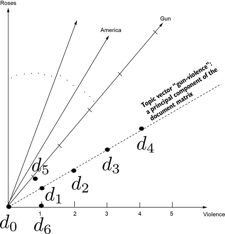 Figure 4.6 Document vectors from our toy dataset d0, ⋯ d6. Each word in the vocabulary corresponds to a separate dimension. Dots show projections of document feature vectors on the plane formed by the axes corresponding to the terms gun(s) and violence.
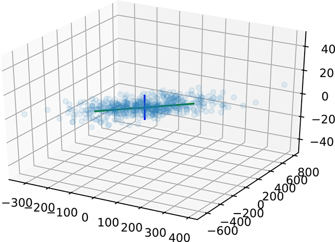 Figure 4.7 Latent semantic analysis. Note that the vertical axis line is actually much smaller than it appears to be in the diagram.
These figures provide a visual understanding of how document vectors are projected onto a lower-dimensional space, revealing the underlying topics and their relationships.
Advanced Example
An advanced example of LSA using SVD is shown in the following listing:
Listing 4.9 LSA using SVD
num_examples = 500
x0 = torch.normal(0, 100, (num_examples,)).round()
random_noise = torch.normal(0, 2, (num_examples,)).round()
x1 = 2*x0 + random_noise
x2 = torch.normal(0, 5, (num_examples,)).round()
X = torch.column_stack((x0, x1, x2))                       #1

                #2
U, S, V_t = torch.linalg.svd(X)                            #3
V = V_t.T                                                  #3
#1 3D dataset: the first two axes are linearly correlated; the third axis has small near-zero random values.
#2 The third singular value is relatively small; we ignore it
#3 The first two principal vectors represent topics. Projecting data points on them yields document descriptors in terms of the two topics.
This example demonstrates the application of LSA to a 3D dataset, where the first two axes are linearly correlated, and the third axis contains small random values. The SVD is used to identify the principal components, which represent the topics, and the data points are projected onto these components to yield document descriptors in terms of the identified topics.