1 Introducing Data Structures
This chapter covers
- Why you should learn about data structures and algorithms
- The difference between algorithms and data structures
- Abstracting a problem
- Moving from problems to solutions
So, you are thinking about learning about algorithms and data structures: excellent decision!
If you are still deciding whether this is for you, I hope this introductory chapter can dispel your doubts and spark your interest on this great topic.
Why should you learn about algorithms? The short answer is: to try and become a better software developer. Knowing about data structures and algorithms is like adding a tool to your tool belt.
Have you ever heard of Maslow’s hammer, aka the law of the instrument? It’s a conjecture, driven by observation, about how people who only know one way to do things, tend to apply what they know to all kind of different situations.
If your tool belt only has a hammer, you will be tempted to treat everything as a nail. If you only know how to sort a list, you will be tempted to sort your tasks list every time you add a new task or have to pick the next one to tackle, and you will never be able to leverage the context to find more efficient solutions.
The purpose of this book is giving you many tools you can use when approaching a problem. We will build upon the basic algorithms normally presented in a computer science 101 course (or alike) and introduce the reader to more advanced material.
After reading this book you should be able to recognize situations where you could improve the performance of your code by using a specific data structure and/or algorithm.
Obviously, your goal should not be remembering by heart all the details of all the data structures we will discuss. We will rather try to show you how to reason about issues, where to find ideas about algorithms that might help you in solving problems. This book will also serve as a handbook, sort of a recipe collection, with indications about some common scenarios that could be used to categorize those problems and the best structures you could use to attack them.
Keep in mind that some topics are quite advanced and, when we delve into the details, it might require a few reads to understand everything. The book is structured in such a way to provide many levels of in-depth analysis, with advanced sections generally grouped together towards the end of each chapter, so if you’d like to get only an understanding of the topics, you are not required delve into the theory.
highlight, annotate, and bookmark
You can automatically highlight by performing the text selection while keeping the alt/ key pressed.
1.1 Data Structures
To start with our journey, we first need to agree on a common language to describe and evaluate algorithms.
Describing them is pretty much a standard process: algorithms are described in terms of the input they take, and the output they provide. Their details can be illustrated with pseudo-code (ignoring implementation details of programming languages), or actual code.
Data structures follows the same conventions, but they also go slightly beyond: we have to describe as well the actions you can perform on a data structure; usually each action is described in term of an algorithm, so with an input, an output, but in addition to those, for DSs we also need to describe side effects, the changes an action might cause to the data structure itself.
To fully understand what this means, we first need to properly define data structures.
1.1.1 Defining a Data Structure
A Data Structure (DS) is a specific solution of organizing data that provides storage for items, and capabilities[1] for storing and retrieving them.
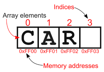
The simplest example of a DS is an array: for instance, an array of characters provides storage for a finite number of characters, and methods to retrieve each character in the array based on its position. Figure 1.1 shows how array = [‘C’, ‘A’, ‘R’] is stored: an array of characters storing the characters C, A, and R, such that for instance array[1] corresponds to the value ‘A’.
Figure 1.1 The (simplified) internal representation of an array.
Each element of the array in the picture corresponds to a byte of memory[2], whose address is shown below it. On top of each element, instead, its index is shown.
An array is stored as a contiguous block of memory, and each element’s address can be obtained by adding its index within the array to the offset of the first element.
For instance, the 4th character of the array (array[3], empty in the figure), has address 0xFF00 + 3 = 0xFF03.
Data structures can be abstract, or concrete.
- An abstract data type (ADT) specify the operations that can be performed on some data and the computational complexity of those operations. No details are provided on how data are stored or how physical memory is used.
- A data structure (DS) is a concrete implementation of the specification provided by an ADT.
Back to our array example, a possible ADT for a static array is, for example: “an array is a container that can store a fixed number of elements, each associated with an index (the position of the element within the array), and access any element by its position (random access)”.
Its implementation, however, needs to take care of details like:
- Will the array size be fixed at creation or can it be modified?
- Will the array be allocated statically or dynamically?
- Will the array host only elements of a single type, or of any type?
- Is it going to be implemented as a raw chunk of memory, or as an object? And what attributes will it hold?
Even for such a basic data structure as arrays, different programming languages make different choices with respect to the questions above. But all of them make sure their version of arrays abides by the array’s ADT we described above.
Another good example to understand the difference might be a stack: we will describe stacks in appendices C and D, but I assume you likely have heard of stacks before.
A possible description of a stack as an ADT is the following: “a container that can store an indefinite number of elements, and can remove elements one at the time, starting from the most recent, according to the inverse order of insertion”.
An alternative description could break down the actions that can be performed on the container: a stack is a container that supports two main methods:
- Insertion of an element.
- Removal of an element: if the stack is not empty, the element that was added the latest will be removed from the stack and returned.
It’s still high level, but clearer and more modular than the previous one.
Either description is abstract enough to make it easily generalizable, allowing to implement a stack in a wide range of programming languages, paradigms and systems[3].
At some point, however, we will have to move to a concrete implementation and then we will need to discuss details like:
- Where are the elements stored?
- o An array?
- o A linked list?
- o A B-tree on disk?
- How do we keep track of the order of insertion? (connected to the previous question)
- Will the max size of the stack be known and fixed in advance?
- Can the stack contain elements of any type or all must be of the same type?
- What happens if removal is called on an empty stack? (for instance, returning null versus throwing an error)
And we could keep going on with questions, but hopefully you get the idea.
1.1.2 Describing a Data Structure
The crucial part of an ADT definition is to list the set operations that it allows. This is equivalent to defining an API[4], a contract with its clients.
Every time you need to describe a data structure, you can follow a few simple steps to make sure to provide a comprehensive and unambiguous specification.
- Specifying its API first, with a focus on the methods' input and output;
- Describing its high-level behavior;
- Describing in detail the behavior of its concrete implementation;
- Analyzing the performance of its methods.
We will use the same workflow for the data structures presented in this book, after describing a concrete scenario in which each data structure is actually used.
Starting in chapter 2, with the description of the first data structure presented, we will also explain in further detail the conventions we use for the API description.
1.1.3 Algorithms and Data Structures: is there a difference?
Yes, they are not exactly the same thing, technically they are not equivalent. Nevertheless, we might sometimes use the two terms interchangeably and, for the sake of brevity, use the term data structure (DS) to intend “a DS and all its relevant methods”.
There are many ways to point out the difference between the two terms, but I particularly like this metaphor: data structures are like nouns, while algorithms are like verbs.
I like this angle because, besides hinting at their different behavior, implicitly reveals the mutual dependency between them. For instance, in English, to build a meaningful phrase, we need both nouns and verbs, subject (or object) and action performed (or endured).
Data structures and algorithms are interconnected, they need each other.
- Data structures are the substrate, a way to organize an area of memory to represent data.
- Algorithms are procedures, sequence of instructions aimed to transform data.
Without algorithms to transform them, data structures would just be bits stored on a memory chip; without data structures to operate on, most algorithms wouldn’t even exist.
Every data structure, moreover, implicitly defines algorithms that can be performed on it: for instance, methods to add, retrieve and remove elements to/from the data structure.
Some data structure is actually defined exactly with the purpose of enabling one or more algorithms to run efficiently on them: think of hash tables and search by key[5].
So, when we use algorithm and data structure as synonyms, it’s just because in that particular context one implies the other: for instance, when we describe a DS, for that description to be meaningful and accurate, we necessarily need to describe its methods (i.e. algorithms).
discuss
1.2 Setting Goals: Your Expectations After Reading this Book
One question you might have, by now, is: “will I ever need to write my own data structures?”.
There is a good chance that you will rarely find yourself in a situation where you don’t have any alternative to writing a data structure from scratch; today it isn’t difficult to find libraries implementing the most common data structures in most programming languages, and usually these libraries are written by experts that knows how to optimize performance or take care of security concerns.
The main goal of this book, in fact, is to give you familiarity with a broad range of tools, and train you to recognize opportunities to use them to improve your code. Understanding how these tools work internally, at least at a high level, is an important part of the learning process. But nevertheless, there are still certain situations in which you might need to get your hands dirty with code, for example if you are using a brand new programming language for which there aren’t many libraries available, or if you need to customize a data structure to solve a special case.
In the end, whether you are going to write your own implementation of data structures really depends on many factors.
First and foremost, how advanced is the data structure you need, and how mainstream is the language you use.
To illustrate this point, let’s take clustering as an example.
If you are working with a mainstream language, for instance in Java or Python it’s very likely that you can find many trusted libraries for k-means, one of the simplest clustering algorithms.
If you are using a niche language, maybe experimenting with a recently created one like Nim or Rust, then it might be harder to find an open source library implemented by a team that has thoroughly tested the code and will maintain the library.
Likewise, if you need an advanced clustering algorithm, like DeLiClu, it will be hard to find even Java or Python implementations that can be trusted to run as part of your application in production.
Another situation in which you might need to understand the internals of these algorithms is when you need to customize one of them, either because you need to optimize it for a real-time environment, because you need some specific property (for example tweaking it to run concurrently and be thread-safe) or even because you need a slightly different behavior.
That said, even focusing on the first part, understanding when and how to use the data structures we present, will be a game changer letting you step up your coding skills to a new level. Let’s use an example to show the importance of algorithms in the real world, and introduce our path in describing algorithms.
settings
1.3 Packing your Knapsack: Data Structures Meet the Real World
Congrats, you have been selected to populate the first Mars colony! Drugstores on Mars are still a bit short of goods… and hard to find. So, you will have, eventually, to grow your own food. In the meantime, for the first few months, you will have goods shipped to sustain you.
1.3.1 Abstracting the Problem Away
The problem is, your crates can’t weight more than 1000 kilograms, and that’s a hard limit.
To make things harder, you can choose only from a limited set of things, already packed in boxes:
- Potatoes, 800 kgs
- Rice, 200 kgs
- Wheat Flour, 400 kgs
- Peanut butter, 10 kgs
- Tomatoes cans, 300 kgs
- Beans, 300 kgs
- Strawberry jam, 50 kgs
You’ll get water for free, so no worries about that, but you can either take a whole crate, or not take it. You’d certainly like to have some choice, and not a ton of potatoes (aka “The Martian” experience).
But, at the same time, the expedition’s main concern is having you well sustained and energetic through your stay, and so the main discriminant to choose what goes on will be the nutritional values. Let’s say the total calories will be a good indicator: table 1.1 sheds a different light on the list of available goods.
Table 1.1 A recap of the available goods, with their weight and calories.
| Food |
Weight (kgs) |
Total calories |
| Potatoes |
800 |
1,501,600 |
| Wheat Flour |
400 |
1,444,000 |
| Rice |
300 |
1,122,000 |
| Beans (can) |
300 |
690,000 |
| Tomatoes (can) |
300 |
237,000 |
| Strawberry jam |
50 |
130,000 |
| Peanut butter |
20 |
117,800 |
So, since the actual content is irrelevant for the decision (despite your understandable protests, mission control is very firm on that point), the only things that matters are the weight and total calories provided, for each of the boxes.
Hence, our problem can be abstracted as “choose any number of items from a set, without the chance to take a fraction of any item, such that their total weight won’t be over 1000 kgs, and in such a way that the total amount of calories is maximized”.
1.3.2 Looking for Solutions
Now that we have stated our problem, we can start looking for solutions.
You might be tempted to start packing your crate with boxes starting from the one with the highest calories value. That would be the potatoes box weighting 800 kgs.
But if you do so, neither rice nor wheat flour will fit in the crate, and their combined calories count exceeds, by far, any other combination you can create within the remaining 200 kgs left. The best value you get with this strategy, is 1,749,400 calories, picking potatoes, strawberry jam and peanut butter.
So, what would have looked like the most natural approach, a greedy[6] algorithm that at each step chooses the best immediate option, does not work. This problem needs to be carefully thought through.
Time for brainstorming. You gather your logistic team and together look for a solution.
Soon enough, someone suggests that, rather than the total calories, you should look at the calories per kg. So, you update table 1.1 with a new column, and sort it accordingly: the result is shown in table 1.2.
Table 1.2 The list in table 1.1, sorted by calories per kg.
| Food |
Weight (kgs) |
Total calories |
Calories per kg |
| Peanut butter |
20 |
117,800 |
5,890 |
| Rice |
300 |
1,122,000 |
3,740 |
| Wheat Flour |
400 |
1,444,000 |
3,610 |
| Strawberry jam |
50 |
130,000 |
2,600 |
| Beans (can) |
300 |
690,000 |
2,300 |
| Potatoes |
800 |
1,501,600 |
1,877 |
| Tomatoes (can) |
300 |
237,000 |
790 |
Then you try to go top to bottom, picking up the food with the highest ratio of calories per unit of weight, ending up with peanut butter, rice, wheat flour and strawberry jam, for a total of 2,813,800 calories.
That’s much better than our first result. It’s clear that this was a step in the right direction. But, looking closely, it’s apparent that adding peanut butter prevented us from taking beans, which would have allowed us to increase the total value of the crate even more. The good news, is that at least you won’t be forced to the Martian’s diet anymore: no potatoes goes on Mars this time.
After a few more hours of brainstorming, you are all pretty much ready to give up: the only way you can solve this is to check, for each item, if you can get a better solution by including it or leaving it out. And the only way you know for doing so, is enumerating all possible solutions, filter out the ones that are above the weight threshold, and pick the best of the remaining ones. This is what’s called a brute force algorithm and we know from Math that it’s a very expensive one.
Since for each item you can either pack it or leave it, the possible solutions are 27=128. You guys are not too keen on going through a hundred solutions, but after a few hours, despite understanding why it’s called brute force, you are totally exhausted, but almost done with it.
Then the news breaks: someone called from the mission control, and following up on complaints from some settlers-to-be, 25 new food items have been added to the list, including sugar, oranges, soy and marmite (don’t ask…).
After checking your numbers everyone is in dismay: now you’d have approximately 4 billion different combinations to check.
1.3.3 Algorithms to the Rescue
At that point, it’s clear that you need a computer program to crunch the numbers and take the best decision.
You write one yourself in the next few hours, but even that takes a long time to run, another couple of hours. Now, as much as you’d like to apply the same diet to all the colonists, turns out some of them have allergies: a quarter of them can’t eat gluten, and apparently many swear they are allergic to marmite. So, you’ll have to run the algorithm again a few times, taking each time into account individual allergies. To make thing worse, mission control is considering adding 30 more items to the list, to make up for what people with allergies will miss. If that happens, we would end up with 62 total possible items, and the program will have to go over several billions of billions of possible combinations. You try that, and after a day the program is still running, nowhere close to termination.
The whole team is ready to give up and go back to the potatoes diet, when someone remembers there is someone in the launch team who had an algorithms book on his desk.
You call them in, and they immediately see the problem for what it is: the 0-1 knapsack problem. The bad news is that it is a NP-complete[7] problem, and this means it is hard to solve, as there is no “quick” (as in polynomial with respect to the number of items) algorithm that computes the optimal solution.
There is, however, also good news: there exist a pseud-polynomial[8] solution, a solution using dynamic programming[9] that takes time proportional to the max capacity of the knapsack, and luckily the capacity of the crate is limited: it takes a number of steps equal to the number of possible values for the capacity filled multiplied by the number of items, so assuming the smallest unit is 1kg, it only takes 1000 * 62 steps. Wow, that’s much better than 262! And, in fact, once you rewrite the algorithm, it finds the best solution in a matter of seconds.
At this time, you are willing to take the algorithm as a black box and plug it in without too many questions. Still, this decision is crucial to your survival… it seems a situation where you could use some deep knowledge of how an algorithm works.
For our initial example, it turns out that the best possible combination we can find is rice, wheat flour and beans, for a total of 3,256,000 calories. That would be quite a good result, compared to our first attempt, right?
You probably had already guessed the best combination, but if it seems too easy in the initial example, where we only have seven items, try the same with hundreds of different products, in a setup closer to the real scenario, and see how many years it takes you to find the best solution by hand!
We could already be happy with this solution, it’s the best we can find given the constraint.
1.3.4 Thinking (literally) out of the Box
But, in our narration, this is the point when the real expert in algorithms comes in. For instance, imagine that a distinguished academic is visiting our facilities while preparing the mission, invited to help with computing the best route to save fuel. During lunch break someone proudly tells her about how you brilliantly solved the problem with packing goods. And then she asks an apparently naïve question: why can’t you change the size of the boxes?
The answer will likely be either that “this is the way it has always been”, or that “items come already packed from vendors, and it would cost time and money to change it”.
And that’s when the expert will explain that if we remove the constrain on the box size, the 0-1 knapsack problem, which is an NP-complete problem, becomes the unbounded knapsack problem, for which we have a linear-time[10] greedy solution that is usually better than the best solution for the 0-1 version.
Translated in human-understandable language, we can turn this problem into one that’s easier to solve and that will allow us to pack the crates with the largest possible total of calories. The problem statement now becomes:
“Given a set of items, choose any subset of items or fraction of items from it, such that their total weight won’t be over 1000 kgs, and in such a way that the total amount of calories is maximized”.
And yes, it is worth to go through the overhead of re-packing everything, because we get a nice improvement.
Specifically, if we can take any fraction of the original weights for each product, we can simply pack products starting from the one with the highest ratio of calories per kg (peanut butter, in this example), and when we get to one box that would not fit in the remaining available space, we take a fraction of it to fill the gap, and repack it. So, in the end we wouldn’t even have to repack all the goods, but just one.
The best solution would then be: peanut butter, rice, wheat flour, strawberry jam, and 230 kilograms of beans, for a total of 3,342,800 calories.
1.3.5 Happy Ending
So, in our story, the future Mars settlers will have greater chances of survival, and won’t go into depression because of a diet only comprising potatoes with a peanut butter and strawberry dip.
From a computational point of view, we moved from incorrect algorithms (the greedy solutions taking the highest total, or highest ratio first), to a correct but unfeasible algorithm (the brute force solution enumerating all the possible combinations) to, finally, a smart solution which would organize the computation in a more efficient fashion.
The next step, as important or even more, brought us to thinking out of the box to simplify our problem, by removing some constraints, and thus finding an easier algorithm and a better solution. This is actually another golden rule: always study your requirements thoroughly, question them and, when possible, try to remove them if that brings you a solution that is at least as valuable, or a slightly less valuable one that can be reached with much lower cost. Of course, in this process, other concerns (like laws and security, at all levels) must be taken into consideration, so some constraints can’t be removed.
In the process of describing algorithms, as we explained in the previous section, we would next describe our solution in details and provide implementation guidelines.
We will skip these steps for the 0-1 knapsack dynamic programming algorithm, both because it’s an algorithm, not a data structure, and it is vastly described in literature. Not to mention that in this chapter its purpose was just illustrating both:
- how important it is to avoid bad choices for the algorithms and data structures we use;
- the process we will follow in the next chapters when it comes to introduce a problem and its solutions.
highlight, annotate, and bookmark
You can automatically highlight by performing the text selection while keeping the alt/ key pressed.
1.4 Summary
- Algorithms should be defined in terms of their input, their output, and a sequence of instructions that will process the input and produce the expected output.
- A data structure is the concrete implementation of an abstract data type, and that it is made of a structure to hold the data and a set of algorithms that manipulate it.
- Abstracting a problem means creating a clear problem statement, and then discussing solution to the problem.
- Packing your knapsack efficiently can be tough (especially if you plan to go to Mars!), but with algorithms and the right data structure, (almost) nothing is impossible!
[1] Specifically, at least one method to add new element to the DS, and one method either to retrieve a specific element or to query the DS.
[2] In modern architectures/languages, it is possible that an array element corresponds to a word of memory rather than a byte, but for the sake of simplicity let’s just assume an array of char is stored as an array of bytes.
[3] In principle, it doesn’t need to be anything computer science: for instance, you could describe as a system a stack of files to be examined, or – a common example in computer science classes – a pile of dishes to be washed.
[4] Application programming interface
[5] you can find more on this topic in appendix C.
[6] A greedy algorithm is a strategy to solve problems that finds the optimal solution by making the locally optimal choice at each step. It can only find the best solution on a small subclass of problems, but it can also be used as a heuristic to find approximate (sub-optimal) solutions.
[7] NP-complete problems are a set of problems for which any given solution can be verified quickly (in polynomial time), but there is no known efficient way to locate a solution in the first place. NP-complete problems, by definition, can’t be solved in polynomial time on a classical deterministic machine (for instance the RAM model we’ll define in next chapter).
[8] For a pseudo-polynomial algorithm, the worst-case running time depends (polynomially) on the value of some inputs, not just the number of inputs. For instance, for the 0-1 knapsack, the inputs are n elements (with weight and value), and the capacity C of the knapsack: a polynomial algorithm depends only on the number n, while a pseudo-polynomial also (or only) depends on the value C.
[9] Dynamic programming is a strategy for solving complex problems with certain characteristics: a recursive structure of subproblems, with the result of each subproblem needed multiple times in the computation of the final solution. The final solution is computed by breaking the problem down into a collection of simpler subproblems, solving each of those subproblems just once, and storing their solutions.
[10] Linear-time, assuming the list of goods is already sorted. Linearithmic otherwise.