Chapter 7. Dijkstra’s algorithm

- We continue the discussion of graphs, and you learn about weighted graphs: a way to assign more or less weight to some edges.
- You learn Dijkstra’s algorithm, which lets you answer “What’s the shortest path to X?” for weighted graphs.
- You learn about cycles in graphs, where Dijkstra’s algorithm doesn’t work.
In the last chapter, you figured out a way to get from point A to point B.
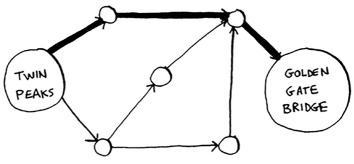
It’s not necessarily the fastest path. It’s the shortest path, because it has the least number of segments (three segments). But suppose you add travel times to those segments. Now you see that there’s a faster path.
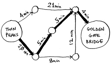
You used breadth-first search in the last chapter. Breadth-first search will find you the path with the fewest segments (the first graph shown here). What if you want the fastest path instead (the second graph)? You can do that fastest with a different algorithm called Dijkstra’s algorithm.
Let’s see how it works with this graph.
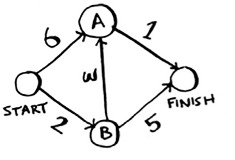
Each segment has a travel time in minutes. You’ll use Dijkstra’s algorithm to go from start to finish in the shortest possible time.
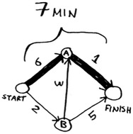
But that path takes 7 minutes. Let’s see if you can find a path that takes less time! There are four steps to Dijkstra’s algorithm:
1. Find the “cheapest” node. This is the node you can get to in the least amount of time.