Suppose a Bayesian model has so much data that thoroughly exploring its posterior takes too long. Variational inference (VI) takes a shortcut: instead of mapping the posterior with many samples, it fits an easier-to-handle distribution to it. Think of a drone photo of a city rather than a walk through every neighborhood—faster, but less detailed. section 6.0 section 6.2
First, choose a family of candidate distributions. Then adjust a candidate’s parameters to make it resemble the target posterior as closely as possible. This turns inference into optimization. The Kullback–Leibler (KL) divergence measures the gap; maximizing the evidence lower bound (ELBO) minimizes that gap. Gradient-based optimization makes fitting practical, and the reparameterization trick handles a difficulty caused by sampling during optimization. section 6.2 section 6.15
Fit a Bayesian linear regression in PyMC
Keep the same model used for MCMC, but replace `pm.sample()` with `vi_approx = pm.fit(n=200_000)`. Then draw from the fitted approximation with `vi_samples = vi_approx.sample(1000, random_seed=0)`. Here, `n` sets the optimization steps. In the illustrated regression, VI and MCMC produce similar posterior means and 94% highest-density intervals, while VI costs less to run. For larger data, `pm.Minibatch` can supply batches during fitting. section 6.9
Speed does not guarantee a faithful picture of uncertainty. A simple candidate may settle on one peak of a posterior with several peaks, or give too little weight to its spread. These risks matter when deciding between VI and MCMC: VI suits large-scale or time-sensitive inference, while MCMC is preferable when faithfully capturing the posterior matters most. section 6.13 section 6.14
Figure 6.6 Demonstrations of pathological behaviors in variational inference. Left: mode-seeking causes the approximator to miss out on other modes. Right: variance underestimation results from the KL divergence formulation.
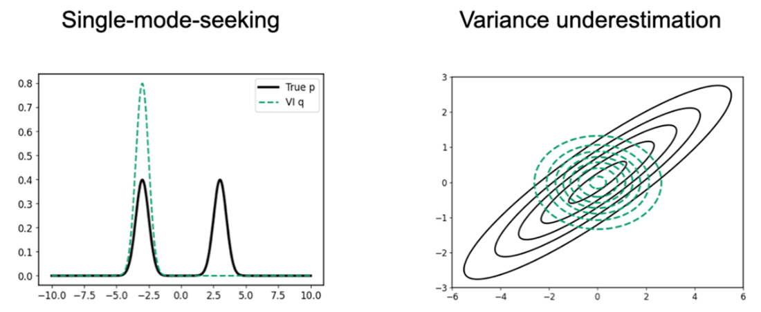
The two panels make the approximation risks visible: one misses a posterior peak; the other captures the center but not enough spread. section 6.13
The same PyMC switch applies to Bayesian neural networks, where a closed-form posterior is unavailable. Minibatches help VI scale, but optimization can be unstable and predictions can miss a trend. Inspecting the ELBO and changing the optimizer or the number of samples used to estimate its gradient can improve the fit; the resulting predictions still deserve comparison with the data. section 10.2 section 10.4


