The autocorrelation function (ACF) measures how strongly a time series is correlated with earlier values of itself at different lags. At lag k, it compares observations k time steps apart. Each coefficient is the covariance of those observations, normalized by their variances. An ACF plot puts lag on the horizontal axis and the corresponding correlation on the vertical axis. section 7.3.7
Use an ACF plot to inspect temporal dependence before fitting a time-series model. A gradual decline across lags suggests that the influence of past values persists; bars outside the plot’s shaded confidence interval suggest significant autocorrelation. ACF measures the overall correlation at each lag. Partial autocorrelation (PACF) instead examines a lag’s direct relationship after accounting for earlier lags. section 7.3.7
Figure 7.3 An ACF plot showing the correlation of a time series with its own past values (lags). The vertical lines represent the autocorrelation coefficients for different lags, with the shaded area indicating the confidence interval. Values outside this shaded region suggest significant autocorrelation, indicating a pattern in the data that could be used for time series forecasting. The gradual decline in the bars signifies the "memory" effect of the time series, where past values influence future observations.
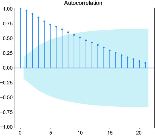
The plotted coefficients, confidence interval, and gradual decline show how to read temporal dependence across lags. section 7.3.7
Check ACF before and after differencing
For closing-price data, reserve April 2024 as the test set and perform preprocessing on the October 2023–March 2024 training set. Plot its ACF with `plot_acf(train)`, then form first differences with `train_diff = train.diff().dropna()` and plot `plot_acf(train_diff)`. Comparing the two plots shows how differencing changes the correlation structure. An augmented Dickey–Fuller test gives a p-value of about 0.576 for the original training series and 1.25 × 10⁻¹⁶ after differencing, providing a separate stationarity check alongside visual inspection. section 7.3.7
>>> fig, axes = plt.subplots(2, 2)     #1
>>> plot_acf(train, ax = axes[0, 0])   #2
>>> axes[0, 0].set_title('ACF - Original')     #3
>>> plot_pacf(train, ax = axes[0, 1])     #4
>>> axes[0, 1].set_title('PACF - Original')     #5
>>> plot_acf(train_diff, ax = axes[1, 0])     #6
>>> axes[1, 0].set_title('ACF - Differenced')   #7
>>> plot_pacf(train_diff, ax = axes[1, 1])    #8
>>> axes[1, 1].set_title('PACF - Differenced')    #9
>>> plt.tight_layout()     #10
>>> plt.show()   #11
The Python listing places ACF and PACF plots for the original and first-differenced training series in one comparison grid. section 7.3.7
ACF and PACF plots also inform decisions about the autoregressive and moving-average components of an ARIMA model after differencing. Interpret nonzero lags when assessing dependence on previous observations: lag zero compares an observation with itself, not with its predecessor. Use the plots with a stationarity check rather than treating a single spike as a complete model-selection rule. section 7.3.7 section 7.3.8
