A stationary time series has statistical properties that remain stable over time. Its mean E(Yₜ) and variance Var(Yₜ) do not depend on t; its autocovariance Cov(Yₜ, Yₛ) depends on the lag |t − s| rather than the particular dates. This stability supports forecasting and statistical inference. section 7.3.5
Figure 7.2 Four illustrative time series charts. Three of the subplots display nonstationary data; in contrast, the plot in the lower-right quadrant displays stationary time series data.
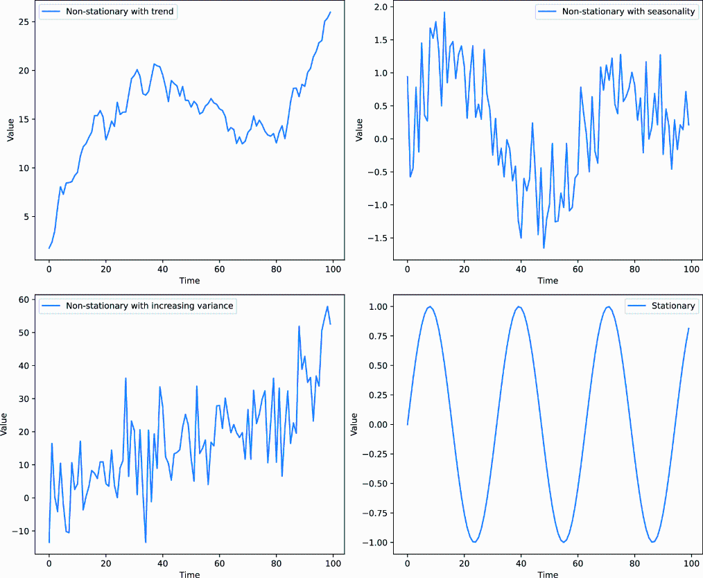
Compare the three nonstationary series with the stationary series in the lower-right chart. A plot is a useful first check, not a substitute for assessing the series used to fit a model. section 7.3.5 section 7.3.7
Stationarity matters when fitting an ARIMA model. Its integration component uses differencing to address nonstationarity. Determine the differencing order d first, then identify the autoregressive order p and moving-average order q. Trends and repeating seasonal patterns can make a series nonstationary; differencing aims to remove them. section 7.3.4 section 7.3.6
First differences of closing prices
For closing prices [173.300247, 171.953735, 173.210495, 174.457260, 177.030579], subtract each price from the next. The first difference is 171.953735 − 173.300247 = −1.346512; the resulting series is [−1.346512, 1.256760, 1.246765, 2.573319]. Five observations yield four differences because the first has no predecessor. In Python, `train_diff = train.diff().dropna()` performs this operation on a training series. section 7.3.6 section 7.3.7
Assess the transformation before fitting:
- Split observations into training and test sets, then assess stationarity and preprocess the training set used for fitting—not the entire series. section 7.3.7
- Inspect the series and its autocorrelation function (ACF) and partial autocorrelation function (PACF) plots. Compare plots before and after differencing to see how the lag-correlation structure changes. section 7.3.7
- Use `statsmodels.tsa.stattools.adfuller` on both versions as a further check. In the closing-price example, the reported p-values are 0.5761116196186049 before differencing and 1.2486140415792743e-16 afterward. section 7.3.7
Figure 7.6 ACF and PACF plots for the original time series (top row) and first-order differenced time series (bottom row). The left column displays the ACF, showing how each observation is correlated with its previous values, whereas the right column presents the PACF, illustrating the direct effect of each lag. These plots are provided to compare the effect of first-order differencing on the time series’ correlation structure.
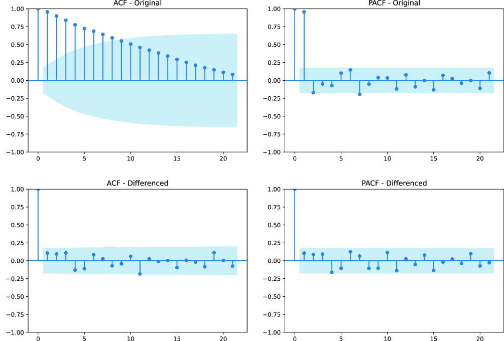
The paired ACF and PACF plots make the effect of first-order differencing on lag correlations visible without treating a transformed plot alone as validation. section 7.3.7
Once the differencing order has been assessed, pass it as d in ARIMA’s `(p, d, q)` order. One illustrated fit uses `ARIMA(train, order=(1, 1, 0))`: one autoregressive lag, first-order differencing, and no lagged forecast-error terms. Stationarity preparation is one part of model selection, not a guarantee of forecast accuracy; predictions still need comparison with held-out observations. section 7.3.9 section 7.3.7
