Differencing replaces a time-series observation with its change from an earlier observation. In ARIMA, it is the integrated (I) component: its job is to address nonstationarity before selecting the autoregressive (AR) and moving-average (MA) components. A stationary series has a mean and variance that remain stable over time, with autocovariance determined by lag rather than calendar position. section 7.3.2 section 7.3.5
First-order differencing subtracts the previous value from the current value: Δyₜ = yₜ − yₜ₋₁. It can reduce a trend; seasonal differencing is another approach for periodic patterns. The order d records how much differencing is used in an ARIMA(p, d, q) model. Choose enough to address nonstationarity, then examine p and q. section 7.3.6 section 7.3.4
Daily closing-price changes
For closing prices [173.300247, 171.953735, 173.210495, 174.457260, 177.030579], first-order differencing produces [−1.346512, 1.256760, 1.246765, 2.573319]. Five prices yield four differences because the first price has no preceding observation to subtract. section 7.3.6
Check the transformation in Python
Split observations before preprocessing and assess the training series, not the entire series. For the closing-price training set: from statsmodels.tsa.stattools import adfuller train_diff = train.diff().dropna() print(adfuller(train)[1]) # 0.5761116196186049 print(adfuller(train_diff)[1]) # 1.2486140415792743e-16 The lower reported ADF p-value after differencing supports reassessing the transformed series as stationary. Plot the series and compare its ACF and PACF before and after differencing; do not rely on the transformation alone as proof. section 7.3.7
Figure 7.6 ACF and PACF plots for the original time series (top row) and first-order differenced time series (bottom row). The left column displays the ACF, showing how each observation is correlated with its previous values, whereas the right column presents the PACF, illustrating the direct effect of each lag. These plots are provided to compare the effect of first-order differencing on the time series’ correlation structure.
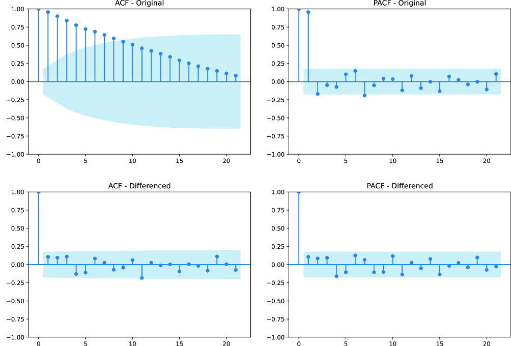
Compare the original and differenced ACF and PACF plots to see how first-order differencing changes the series’ lag-correlation structure. section 7.3.7
If the ACF still decays slowly or correlations persist across many lags, consider whether more differencing is needed. If the series appears stationary but its PACF has significant spikes at particular lags, consider increasing the AR order instead. Exponential smoothing offers a different forecasting approach based on weighted past observations rather than ARIMA’s differencing step. section 7.3.8 section 7.4.3
