Automatic differentiation computes derivatives, or gradients, of tensor-based computations without requiring manual calculus for each new function. In PyTorch, operations build a record of the computation; calling `.backward()` traverses that record and calculates gradients for tracked tensors. section 1.3 section 1.3.2
Gradients support optimization because they describe how a loss changes. For a scalar function f(x), the derivative’s sign indicates which direction reduces the function, while its magnitude indicates the local rate of change. Gradient descent updates the current value in the opposite direction: x₍ₖ₊₁₎ = xₖ − ηf′(xₖ), where η is the learning rate. section 1.3.1 section 1.3.3
A minimal PyTorch workflow follows these steps:
- Create a tensor with `requires_grad=True` so PyTorch tracks operations involving it. section 1.3.2
- Evaluate a function or model loss using PyTorch operations; the result carries a computation history such as `grad_fn`. section 1.3.2
- Call `.backward()` on the scalar result to compute gradients, then read the original tensor’s `.grad` value. section 1.3.2
- Update parameters in the opposite gradient direction, control the step with a learning rate, and clear stored gradients before the next iteration. section 1.3.3
Minimizing a quadratic
For f(x) = (x − 2)², start with x = −3.5 and mark it for gradient tracking. Evaluate `value = f(x)`, call `value.backward()`, and obtain x.grad = −11, the derivative at the starting point. Repeatedly update x with `x.data -= eta * x.grad`, reset `x.grad`, and stop when successive values differ by less than ε. With η = 0.1, the iteration reaches approximately x = 2, where f(x) = 0. A step that is too small converges slowly; a step that is too large can diverge. section 1.3.2 section 1.3.3
For neural networks, the scalar loss replaces the toy function. The model produces predictions, the loss compares predictions with correct answers, and automatic differentiation supplies a gradient for every registered parameter. The resulting training loop uses those gradients to reduce loss and improve predictions. The gradient is a tensor-shaped collection of derivatives rather than a single number. section 2.1 section 2.1.1
Figure 1.7 Three examples of how the learning rate η (also called step size) impacts learning. On the left, η is smaller than necessary. This still reaches the minimum but takes more steps than needed. If we knew the perfect value of η, we could set it just right, to take the smallest number of steps to the minimum value (middle). On the right, η is too big, which causes divergence. We never reach the solution!
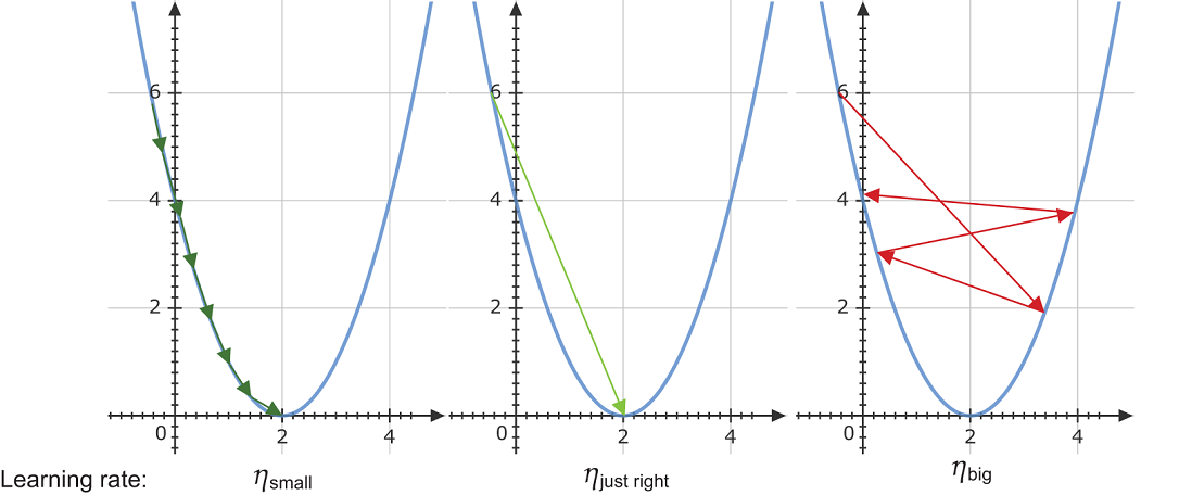
Compare learning-rate choices visually: undersized steps take longer, a suitable step reaches the minimum efficiently, and oversized steps cause divergence. section 1.3.3