Automatic differentiation

As explained in Math and Architectures of Deep Learning

A method for mechanically computing derivatives of functions by tracing elementary operations.

Automatic differentiation mechanically computes derivatives by tracing the elementary operations in a function. It replaces hand-derived, closed-form gradients when models contain many parameters or nonlinear functions. In PyTorch, specifying the model function lets Autograd construct and use the required gradient computation. section 3.5.2 section 3.5.1

Set requires_grad = True on variables whose gradients should be tracked. PyTorch then maintains a computation graph as expressions are created. Calling backward() on a loss traverses that graph and computes gradients for the tracked parameters. section 3.5.2 section 8.5

A typical gradient-based training loop is:

• Run the model’s forward pass to produce predictions. section 8.5
• Evaluate a loss function such as mean squared error. section 8.5
• Call loss.backward() to compute parameter gradients automatically. section 8.5
• Use an optimizer’s step operation to update weights and biases. section 8.5

From linear regression to neural-network training

For a linear model y_pred = b + w*x, Autograd computes gradients without explicitly writing the formulas for w and b. The same mechanism extends to a two-layer PyTorch network: compute predictions, evaluate MSELoss, clear previous gradients, call mse_loss.backward(), and run optimizer.step(). Repeating this loop reduces the loss and brings predictions closer to the observed targets.

Figure 3.10 Autograd analysis

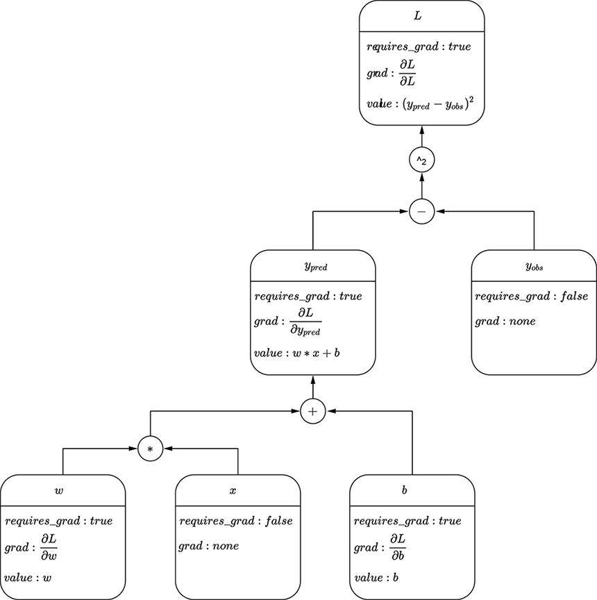
Use the computation-graph figure to connect tracked operations with the gradients produced by Autograd. section 3.5.2

How Math and Architectures of Deep Learning covers it

How deep it goes

Explains requires_grad, computation graphs, backward(), and optimizer updates, but does not derive Autograd internals.

Examples

Uses a noisy linear model and a demand-prediction neural network trained with mean squared error.

What you can do after

Apply it via PyTorch Autograd to compute gradients and train linear or neural-network models.

How it connects

Connects computation graphs with backpropagation, loss functions, gradients, gradient descent, and optimizers.

liveBookmanning.com

Read Math and Architectures of Deep Learning on liveBook Get the book at manning.com

Also explained in

• 

  liveBookmanning.com
  Inside Deep Learning: Math, Algorithms, ModelsA mechanism for computing derivatives of model computations automatically, used here to support training of networks with registered parameters.
• 

  liveBookmanning.com
  Deep Learning with JAXA technique for computing exact derivatives of code-expressed computations by systematically applying differentiation rules to the program structure.
• 

  liveBookmanning.com
  Deep Learning with R, Third EditionAutomatic differentiation computes exact derivatives of programs composed of differentiable operations by systematically applying the chain rule.
• 

  liveBookmanning.com
  Deep Learning with PyTorch, Second EditionA technique for automatically computing derivatives needed for training neural networks.
• 

  liveBookmanning.com
  Deep Learning with Python, Third EditionA mechanism that programmatically computes exact derivatives of recorded operations by applying the chain rule to a computation graph.

Compare how 6 books explain automatic differentiation →

Related concepts

• PyTorchused by · PyTorch is an open-source machine-learning framework for Python that provides tensor computation, automatic differentiation, and tools for building and training neural networks.
• JAXused by · JAX is a Python library for high-performance array-based numerical computing with composable transformations including automatic differentiation, compilation, vectorization, and parallelization.
• derivativeproduces · A derivative is a mathematical quantity that measures the instantaneous rate of change of a function with respect to an input variable.
• computation graphuses · A computation graph is a directed graph whose nodes represent computational operations or values and whose edges represent data dependencies between them.
• gradientproduces · A gradient is the vector of partial derivatives of a scalar function with respect to its variables, indicating its local rate and direction of change.
• jax.gradimplemented by · jax.grad is a JAX transformation that creates a function computing derivatives, typically gradients of a scalar-output function with respect to specified inputs.

This explainer was generated by Manning's knowledge graph from the text of Math and Architectures of Deep Learning. The section links point to the parts of the book it draws on.