Gradient boosting

As explained in Ensemble Methods for Machine Learning

Gradient boosting is an ensemble-learning technique that sequentially adds models trained to correct the errors of prior models using gradient-based optimization.

Gradient boosting builds a strong predictor by adding weak models one at a time. Each new model concentrates on what the current ensemble still gets wrong, so the sequence improves predictions stage by stage rather than training members independently. Its central idea is simple: use each example’s loss-derived error signal to decide what the next weak learner should learn. section 5.0 section 1.5

A residual is the gap between a true label and the model’s current prediction. Large residuals mark examples needing more attention; small residuals mark examples already fit well. For squared loss, the negative loss gradient equals the residual. More generally, gradient boosting trains weak learners to approximate the loss gradient, making the method applicable to classification, regression, and ranking through a suitable loss function. section 5.2.1 section 5.0

A basic gradient-boosting procedure is:

• Initialize the ensemble prediction with a constant value. section 5.2.2
• Compute negative residuals from the current predictions for all training examples. section 5.2.2
• Fit a weak regression tree to those residuals, using it as an approximation to the negative gradient. section 5.2.2 section 5.2.1
• Choose a step length, then add the weighted tree to the current ensemble. section 5.2.2
• Repeat for a fixed maximum number of iterations and sum the weighted tree predictions at inference time. section 5.2.2

Figure 5.9 Comparing gradient descent (left) to gradient boosting (right). At iteration t, gradient descent updates the model using the negative gradient, -g_t. At iteration t, gradient boosting approximates the negative gradient by training a weak regressor, h_t, on the negative residuals -r^t_i. The step length α_t in gradient descent is equivalent to the hypothesis weight of each base estimator in a sequential ensemble.

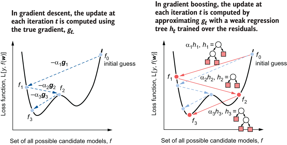
Compare the update rule with gradient descent: gradient descent adds a gradient vector, while gradient boosting adds a weak regressor trained to approximate that update. section 5.2.1

Gradient boosting differs from AdaBoost in how it communicates mistakes to the next learner. AdaBoost increases the weights of misclassified examples. Gradient boosting instead supplies residuals directly and fits a regressor to them. Both are sequential boosting methods, but residuals carry both the size and, in regression, the direction of the correction: positive residuals indicate underprediction and negative residuals indicate overprediction. section 5.2.1 section 7.3

Two-moons classifier from scratch

With squared loss, initialize all predictions to zero, calculate residuals, and fit shallow decision-tree regressors in sequence. On a noisy two-moons classification data set, a 10-estimator implementation predicts by summing weighted tree outputs and taking their sign; the reported test error is 6%. Iteration visualizations show residuals changing as successive trees repair the ensemble’s remaining errors. section 5.2.2 section 5.2.2

For larger practical workloads, histogram-based tree learning trades some exactness for faster training. LightGBM provides gradient boosting with efficient parallel and GPU-oriented training, support for varied and custom losses, and controls for overfitting such as learning rate and early stopping. Important tuning areas include tree depth, subsampling, L1/L2 regularization, and loss-specific parameters; randomized search with cross-validation can be preferable to exhaustive grid search. section 5.6 section 7.3.2

Robust regression with LightGBM

An LGBMRegressor configured with Huber loss can model continuous labels while reducing the influence of large errors. A randomized cross-validation search tunes alpha, learning rate, subsampling, tree depth, and L1/L2 regularization; an evaluation set supports performance monitoring. In the AutoMPG example, the selected model reports test MSE 0.0951 and test MAE 0.2250. section 7.3.2

How Ensemble Methods for Machine Learning covers it

How deep it goes

Explains residual intuition, gradient-descent correspondence, stepwise training, from-scratch trees, and LightGBM tuning.

Examples

Uses noisy two-moons classification and AutoMPG regression with Huber-loss LightGBM.

What it assumes

Reinforces boosting, loss functions, residuals, and gradient descent before implementing tree ensembles.

What you can do after

Build it from scratch with weak regression trees, residual fitting, line search, and additive prediction updates.

How it connects

Connects gradient boosting to AdaBoost, gradient descent, residuals, loss functions, regression trees, LightGBM, and XGBoost.

liveBookmanning.com

Read Ensemble Methods for Machine Learning on liveBook Get the book at manning.com

Also explained in

• 

  liveBookmanning.com
  Machine Learning for Tabular Data: XGBoost, Deep Learning, and AIA decision-tree ensemble model built by sequentially adding trees to optimize a predictive loss using gradient-based optimization.
• 

  liveBookmanning.com
  Grokking Machine LearningAn ensemble model that sequentially combines decision trees, with each tree improving the ensemble's fit to the data.
• 

  liveBookmanning.com
  Machine Learning System DesignA gradient-boosting model is an ensemble model built by sequentially fitting weak predictive models to reduce the errors of the current ensemble.
• 

  liveBookmanning.com
  The Art of AI Product DevelopmentA gradient boosting algorithm builds an ensemble model by sequentially adding weak predictive models that reduce errors made by the existing ensemble.

Compare how 5 books explain gradient boosting →

Related concepts

• XGBoostimplemented by · XGBoost is an open-source software library for efficient gradient-boosted decision-tree algorithms used in supervised machine learning.
• Newton boostingcontrasts with · Newton boosting is a boosting approach that uses first- and second-order loss information to construct successive learners.
• ensemblekind of · An ensemble is a technique that combines or considers outputs from multiple models or component methods collectively to produce or assess a joint result.
• random forestalternative to · A random forest is an ensemble model that combines predictions from multiple decision trees built with randomized data samples, feature selections, or both.
• decision treehas part · A decision tree is a branching structure that represents sequential tests or choices, with paths leading to outcomes, predictions, or actions.
• language modelkind of · A language model is a computational model that represents patterns in linguistic tokens to estimate sequence probabilities and predict or generate language from context.

This explainer was generated by Manning's knowledge graph from the text of Ensemble Methods for Machine Learning. The section links point to the parts of the book it draws on.