Gradient boosting

As explained in Machine Learning for Tabular Data: XGBoost, Deep Learning, and AI

A decision-tree ensemble model built by sequentially adding trees to optimize a predictive loss using gradient-based optimization.

Gradient boosting is a decision-tree ensemble for tabular prediction. It starts with a simple constant prediction and adds trees one at a time. Each new tree learns a correction to the current model’s errors, moving the ensemble toward a lower predictive loss. The result combines the flexible, rule-based splits of decision trees with a gradient-descent-style optimization process. section 5.2 section 5.2.1

This makes gradient-boosted decision trees (GBDTs) a strong default for many heterogeneous business datasets containing numeric and categorical-style inputs, missing values, nonlinear effects, noise, and outliers. They are widely used for classification, regression, click prediction, and ranking. Performance depends on tuning, but standard tabular problems often favor GBDTs over neural networks, support vector machines, random forests, and bagging ensembles. section 5.2 section 5.2.3

A boosted model is built from a few linked parts:

• An initial prediction, such as the target average or a starting estimator. section 5.2.1 section 5.3
• A sequence of regression trees, including when the final task is binary classification. section 5.2.1
• A loss gradient or residual-like correction that tells each next tree what to improve. section 5.2 section 5.2.2
• A learning rate that scales every tree’s contribution and trades off against the number of trees. section 5.2.1 section 6.3.5
• Tree-complexity settings, such as depth and minimum leaf size, that control fit versus overfitting risk. section 5.3 section 6.3.5

Classifying higher-priced Airbnb listings

For a binary task that predicts whether an Airbnb NYC listing is above the median price, a custom classifier begins from the target prevalence, repeatedly fits DecisionTreeRegressor models to corrections, and sums their scaled outputs. A configuration with 300 estimators, a 0.1 learning rate, depth 4, and minimum leaf size 3 achieved 0.82503 accuracy on a held-out test set. A Scikit-learn pipeline using GradientBoostingClassifier and five-fold cross-validation reported mean accuracy of 0.826, with fitting taking 16.48 seconds and prediction 0.07 seconds. section 5.2.1 section 5.3

For binary classification, boosted trees can model probability predictions by working with logits: probabilities are mapped onto an unbounded log-odds scale, trees fit corrections there, and the sigmoid maps the final result back to the 0–1 range. This direct optimization can yield probability estimates that rarely need later calibration. A regression-style treatment of probabilities, however, can produce values outside the 0–1 boundary. section 5.2.1 section 5.2.2

Gradient boosting is not automatically simple or cheap. Many hyperparameters interact, and more trees can make computation costly. Lower learning rates generally require more trees; deeper trees add complexity and can increase overfitting risk, so reducing the learning rate as depth rises is advisable. Although trees capture nonlinear relationships, their binary splits can be rough approximators; known nonlinearities and interactions may benefit from explicit transformations, binning, or precomputed interaction features. section 5.6 section 6.1.4 section 6.3.5

Figure 5.5 How gradient descent works with boosted trees

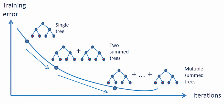
Use the diagram to connect the abstract optimization idea to the practical sequence of trees: each added tree contributes a scaled correction to the ensemble prediction. section 5.2

Common implementations include Scikit-learn’s gradient boosting, XGBoost, and LightGBM. Scikit-learn provides detailed control of individual-tree settings and initialization, while newer histogram-based approaches aim to improve speed. XGBoost adds more complex Newton-style optimization and supports custom objectives, GPU training, missing values, monotonicity constraints, and feature-interaction constraints. XGBoost and LightGBM also expose tree structures that can be saved, plotted, and traversed to inspect split features, thresholds, gains, and leaves. section 5.3 section 5.6 section 6.4.2

Choosing between gradient boosting and deep learning is empirical rather than absolute. Gradient boosting is a leading approach for ordinary tabular problems, but deep learning can be preferable in some cases. Comparing predictive quality, inference time, maintenance cost, clarity to stakeholders, and postdeployment stability helps make the choice. Averaging a boosted model with a deep learning model can improve predictions when their different estimation approaches produce complementary errors. section 12.0 section 12.6

How Machine Learning for Tabular Data: XGBoost, Deep Learning, and AI covers it

How deep it goes

Explains sequential corrections, logits, probabilities, tree controls, tuning tradeoffs, and inspectable XGBoost and LightGBM structures.

Examples

Demonstrates Airbnb NYC price classification, predicted-probability histograms, regression behavior, Scikit-learn cross-validation, and XGBoost and LightGBM tree extraction.

What it assumes

Builds from decision trees, linear models, regularization, and gradient descent while introducing boosted-tree mechanics through an implementation.

What you can do after

Apply it via Scikit-learn, XGBoost, or LightGBM to train, tune, evaluate, inspect, and compare tabular predictive models.

How it connects

Connects decision trees, gradient descent, regression trees, logits, sigmoid, AdaBoost, XGBoost, LightGBM, partial dependence plots, and deep learning.

liveBookmanning.com

Read Machine Learning for Tabular Data: XGBoost, Deep Learning, and AI on liveBook Get the book at manning.com

Also explained in

• 

  liveBookmanning.com
  Ensemble Methods for Machine LearningGradient boosting is an ensemble-learning technique that sequentially adds models trained to correct the errors of prior models using gradient-based optimization.
• 

  liveBookmanning.com
  Grokking Machine LearningAn ensemble model that sequentially combines decision trees, with each tree improving the ensemble's fit to the data.
• 

  liveBookmanning.com
  Machine Learning System DesignA gradient-boosting model is an ensemble model built by sequentially fitting weak predictive models to reduce the errors of the current ensemble.
• 

  liveBookmanning.com
  The Art of AI Product DevelopmentA gradient boosting algorithm builds an ensemble model by sequentially adding weak predictive models that reduce errors made by the existing ensemble.

Compare how 5 books explain gradient boosting →

Related concepts

• XGBoostimplemented by · XGBoost is an open-source software library for efficient gradient-boosted decision-tree algorithms used in supervised machine learning.
• Newton boostingcontrasts with · Newton boosting is a boosting approach that uses first- and second-order loss information to construct successive learners.
• ensemblekind of · An ensemble is a technique that combines or considers outputs from multiple models or component methods collectively to produce or assess a joint result.
• random forestalternative to · A random forest is an ensemble model that combines predictions from multiple decision trees built with randomized data samples, feature selections, or both.
• decision treehas part · A decision tree is a branching structure that represents sequential tests or choices, with paths leading to outcomes, predictions, or actions.
• language modelkind of · A language model is a computational model that represents patterns in linguistic tokens to estimate sequence probabilities and predict or generate language from context.

This explainer was generated by Manning's knowledge graph from the text of Machine Learning for Tabular Data: XGBoost, Deep Learning, and AI. The section links point to the parts of the book it draws on.