Brute-force search explores possibilities without using problem-specific knowledge to favor states that appear closer to a goal. In graph search, this is called blind or uninformed search. It can navigate a maze, solve a puzzle, or find a route using a fixed rule and a way to recognize the goal. section 3.2 section 4.1
The rule determines what gets explored next. Blind does not mean arbitrary: these algorithms systematically examine a graph, and some use known edge costs. What they lack is a goal-directed estimate, such as a heuristic predicting the remaining distance. section 3.2 section 4.1
Common rules produce different search behavior:
- Breadth-first search (BFS) explores one level before the next; depth-first search (DFS) follows a branch before backtracking. section 3.6
- Depth-limited search caps DFS exploration; iterative deepening raises that cap until it reaches the goal. section 3.6
- Dijkstra’s algorithm finds shortest paths in weighted graphs with non-negative edge costs. Uniform-cost search selects by lowest cumulative cost; with equal edge costs, it is equivalent to BFS. section 3.6
- Bidirectional search explores from both the start and the goal. section 3.6
Stopping at the first feasible solution need not give the best one. An exhaustive brute-force strategy instead checks feasible solutions and compares them, but broader exploration has time and memory costs. Choose a rule according to the goal, available edge costs, and acceptable time–space trade-off. section 3.2 section 3.6
Routing without a direction hint
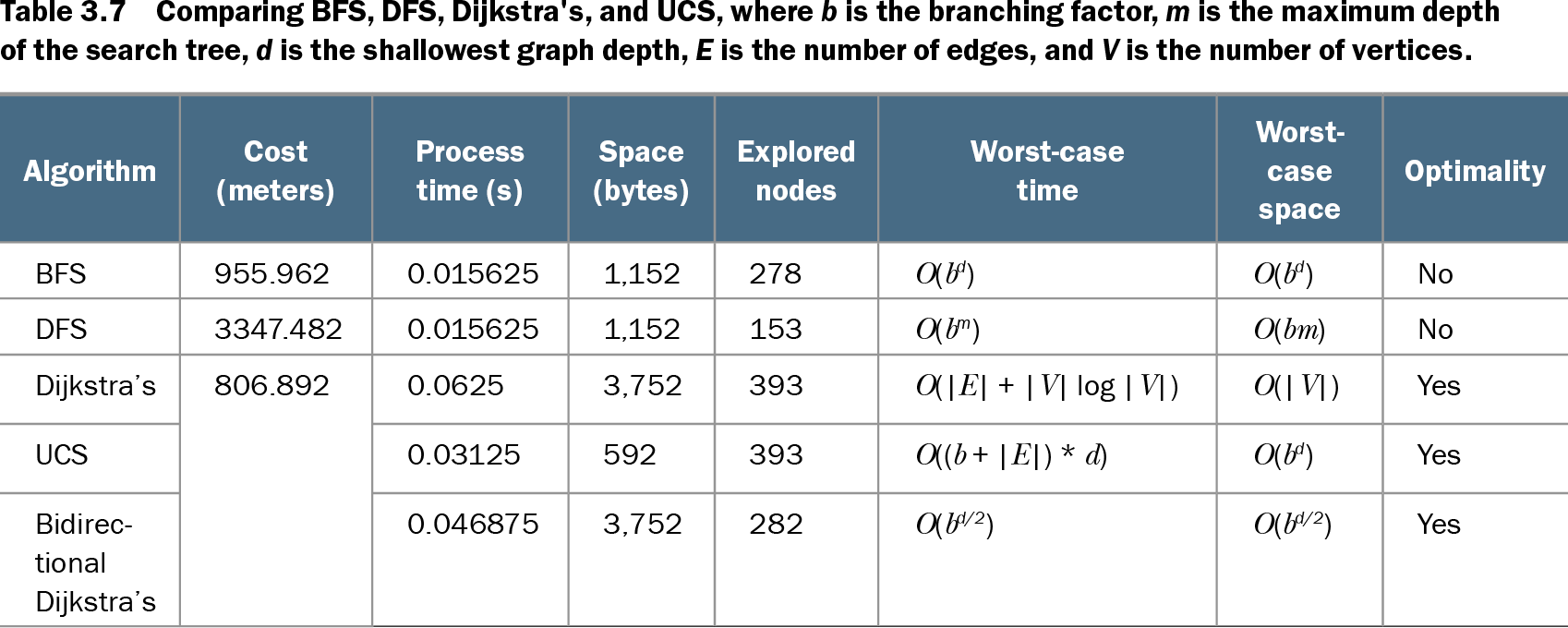
Suppose you need a route across Toronto but do not know which direction leads toward the destination. Apply BFS, DFS, Dijkstra’s algorithm, uniform-cost search, or bidirectional Dijkstra’s to the same street graph and compare route length, explored nodes, time, and memory. In the reported comparison, BFS and DFS found longer routes than the weighted shortest-path methods. For map graphs, handle parallel edges and self-loops carefully: an unsuitable parallel edge can inflate route length, while a self-loop can break route reconstruction. section 3.5
Table 3.7 Comparing BFS, DFS, Dijkstra's, and UCS, where b is the branching factor, m is the maximum depth of the search tree, d is the shallowest graph depth, E is the number of edges, and V is the number of vertices. (view table figure)
| Algorithm |
Cost (meters) |
Process time (s) |
Space (bytes) |
Explored nodes |
Worst-case time |
Worst-case space |
Optimality |
|---|---|---|---|---|---|---|---|
| BFS |
955.962 |
0.015625 |
1,152 |
278 |
O(bd) |
O(bd) |
No |
| DFS |
3347.482 |
0.015625 |
1,152 |
153 |
O(bm) |
O(bm) |
No |
| Dijkstra’s |
806.892 |
0.0625 |
3,752 |
393 |
O(|E| + |V| log |V|) |
O(|V|) |
Yes |
| UCS |
0.03125 |
592 |
393 |
O((b + |E|) * d) |
O(bd) |
Yes |
|
| Bidirectional Dijkstra’s |
0.046875 |
3,752 |
282 |
O(bd/2) |
O(bd/2) |
Yes |
Compare the routing algorithms’ measured costs, explored nodes, resource use, and stated optimality when choosing a search rule. section 3.5