A bigger model is not necessarily a more complicated explanation. Model size describes how much capacity a network has; model complexity can instead describe how much information its learned parameters require. This distinction matters when a network fits its training data but must still predict well on new examples. section 8.4.1 section 8.5.3
Geoffrey Hinton and Drew van Camp made complexity a training cost. Their minimum description length objective counts the bits needed to specify a network’s weights plus the bits needed to correct its errors on the training data. A fit that depends on unusually precise weights is expensive; a less precise fit can be cheaper, provided its prediction errors do not cost too much. In their method, each weight has a Gaussian distribution, and its information cost is measured by its Kullback–Leibler divergence from a prior. Training adjusts both the weight means and their variability while minimizing the combined cost. section 8.4.1
A small-data test
On a peptide activity task with 105 training examples, Hinton and van Camp used a network with 521 weights. Its test relative error was 0.286 with the description-length penalty, versus 0.967 without it; a tuned weight-decay comparison reached 0.317. Charging for weight information helped this oversized network avoid fitting noise. section 8.4.2
Double descent offers a second reason not to equate size with a simple complexity ranking. Test error can rise when a model becomes just large enough to fit the training set, then fall as it grows further. Near that interpolation threshold, a fit can be brittle and sensitive to noisy labels. A larger model has more possible fits, allowing stochastic gradient descent to find one that also performs well on the data distribution. Capacity has increased, but the resulting explanation need not be more complex. section 8.5.3
Figure 8.10 Test (solid line) and training (dashed line) errors for ResNet as the width increases. A peak near the interpolation threshold (dashed line; shaded “critical” band) illustrates double descent, in which error rises as the model fits the data, then falls again for larger widths. Used with permission granted by the lead author (Preetum Nakkiran).
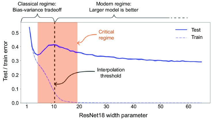
The ResNet width plot makes the distinction visible: test error peaks near the interpolation threshold before falling at larger widths. section 8.5.3
Complexity also names visible structure outside modeling. Cream mixing into coffee starts in distinct layers, forms intricate swirls, then becomes uniform. Its complexity peaks between the orderly beginning and the high-entropy end, even as entropy keeps increasing. That use of complexity concerns patterns in a system, not the bit cost of a network’s weights. section 8.1 section 8.4.1