Constant function

As explained in Bayesian Optimization in Action

A constant mean function is a Gaussian-process mean function that assigns the same expected value to every input.

A constant mean function assigns the same expected value to every input in a Gaussian process. It provides a simple prior prediction before observations are incorporated, while the covariance function models relationships between inputs. section 3.2

Use a nonzero constant when prior knowledge suggests that objective values occupy a particular range. Accuracy commonly lies between 0 and 1, while housing prices are positive, so a positive constant can be more appropriate than a zero mean. section 3.3.2 section 3.2

Choose and train the constant mean as follows:

• Treat the constant as a candidate expected objective value, such as 0 or 2. section 3.3.2
• Compare candidates using the exact marginal log likelihood, which measures how well the GP explains its training data. section 3.3.2
• Optimize the mean constant with gradient descent, minimizing negative marginal log likelihood alongside other GP hyperparameters when appropriate. section 3.3.2 section 12.1.2
• Switch both the model and likelihood from training mode to evaluation mode before making predictions. section 12.1.2

Comparing zero and positive means

Two otherwise comparable GP models use constant means of 0 and 2. The model with mean 2 has higher log likelihood, and its predictions revert toward 2 away from observed data, indicating a better fit for the training observations. section 3.3.2

Figure 3.6 GP predictions, given two different constant mean functions. The value 2 gives a higher likelihood value than the value 0, indicating the former mean function is a better fit than the latter.

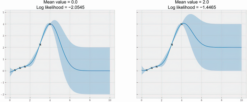
Compare GP predictions produced by two constant mean values and inspect how the better likelihood changes prior reversion. section 3.3.2

In GPyTorch, implement the mean with gpytorch.means.ConstantMean. A regular GP can combine it with an RBF or Matérn kernel and a ScaleKernel, then learn the constant through Adam and the marginal-log-likelihood objective. section 12.1.2 section 7.5

How Bayesian Optimization in Action covers it

How deep it goes

Defines prior behavior, compares candidate values with marginal likelihood, and demonstrates gradient-based fitting without deriving Gaussian-process internals.

Examples

Uses housing prices, model accuracy, zero-versus-two mean predictions, and four-dimensional airplane-design optimization.

What it assumes

Assumes basic Gaussian-process and gradient-descent familiarity while motivating mean functions through objective ranges and simple prediction comparisons.

What you can do after

Apply it via GPyTorch by defining ConstantMean and fitting its constant with Adam and exact marginal log likelihood.

How it connects

Connects mean functions with covariance functions, Gaussian processes, marginal likelihood, gradient descent, kernels, and Bayesian optimization.

liveBookmanning.com

Read Bayesian Optimization in Action on liveBook Get the book at manning.com

Related concepts

• Gaussian processused by · A Gaussian process is a probability distribution over functions in which every finite collection of function values has a joint Gaussian distribution.
• mean functionkind of · A mean function maps an input to the expected value of a random function before conditioning on observed data.
• linear regressioncontrasts with · Linear regression is a statistical modeling method that estimates a continuous response as a linear combination of predictor variables and fitted coefficients.
• gradient descentused by · Gradient descent is an iterative optimization method that updates parameters opposite the gradient of an objective function to reduce its value.
• RAM modelused by · The RAM model is an abstract computational model with a processor, randomly accessible memory, and basic constant-time instructions for analyzing algorithm complexity.

This explainer was generated by Manning's knowledge graph from the text of Bayesian Optimization in Action. The section links point to the parts of the book it draws on.