Mean function

As explained in Bayesian Optimization in Action

A mean function maps an input to the expected value of a random function before conditioning on observed data.

A mean function maps each input x to the expected value of f(x). In a Gaussian process (GP), it replaces the fixed mean vector of a multivariate normal distribution, letting the model express expectations at any location in an input domain. section 2.3

Think of it as a first guess about an unknown objective before observations are considered. It controls the broad expected behavior or shape of the function, while the covariance function controls relationships between points, smoothness, and variability. This prior knowledge is especially valuable when evaluating the objective is expensive. section 3.0 section 3.2

Common choices encode different prior expectations:

• Zero mean: predict zero by default when no useful prior information is available. Far from observed data, posterior predictions revert toward this prior mean. section 3.3.1
• Constant mean: represent a known typical output level, such as positive housing prices. Its constant can be learned by maximizing marginal log likelihood. section 3.3.2
• Linear or quadratic mean: impose corresponding general trends on GP predictions when prior knowledge supports them. section 3.2 section 3.6

Housing-price prior

For living area and price, prices are known to be positive and generally increase with area. A zero mean supplies no such expectation; a positive constant mean gives a more plausible baseline in unobserved regions. Comparing marginal likelihoods can favor a constant of 2 over zero when it explains the observed prices better. section 3.3 section 3.3.2

In GPyTorch, the mean and covariance are modules evaluated in parallel inside a GP model’s forward method; their outputs form a multivariate normal distribution. `ZeroMean()` gives a fixed zero prior, while `ConstantMean()` starts at zero by default but exposes a trainable constant. section 2.4.2 section 3.3.1

Figure 2.17 Predictions made by a prior GP with a zero mean and RBF kernel. While the mean and CI are constant, individual samples exhibit complex, nonlinear behaviors.

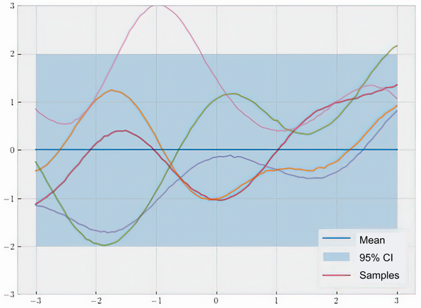
Compare the constant prior mean and confidence interval with nonlinear sampled functions: the mean is an expectation, not a typical individual realization. section 2.4.4

After conditioning on data, the posterior mean can smoothly interpolate observations, but its behavior away from them remains influenced by the prior mean. The same idea applies to multidimensional inputs as long as the mean and covariance functions accept them; predictive means can then be displayed as heat maps. section 3.3.1 section 2.4.5

How Bayesian Optimization in Action covers it

How deep it goes

Defines input-to-expectation behavior, contrasts it with covariance, and implements zero and optimized constant means without deriving GP inference.

Examples

Uses housing prices versus living area, zero and constant priors, predictive plots, sampled functions, and two-dimensional heat maps.

What it assumes

Assumes familiarity with GP models and multivariate normal distributions while defining the mean function directly.

What you can do after

Apply it via GPyTorch to set zero or constant priors and optimize a constant mean with marginal likelihood.

How it connects

Connects Gaussian processes to covariance functions, prior knowledge, posterior predictions, marginal likelihood, and gradient descent.

liveBookmanning.com

Read Bayesian Optimization in Action on liveBook Get the book at manning.com

Related concepts

• Gaussian processpart of · A Gaussian process is a probability distribution over functions in which every finite collection of function values has a joint Gaussian distribution.
• prior knowledgeused by · Prior knowledge is information, beliefs, skills, or assumptions available to an agent before it encounters a task or incorporates new observations.
• constant functionincludes · A constant function produces the same output value for every input in its domain.
• linear regressionincludes · Linear regression is a statistical modeling method that estimates a continuous response as a linear combination of predictor variables and fitted coefficients.
• quadratic mean functionincludes · A quadratic mean function maps an input to an expected value represented by a second-degree polynomial with learned coefficients.

This explainer was generated by Manning's knowledge graph from the text of Bayesian Optimization in Action. The section links point to the parts of the book it draws on.