Count data uses a target label that records how many events or items occurred: doctor visits, insurance claims, crimes, births, deaths, or casual bike users. Unlike a continuous target, a count is discrete and nonnegative. A regression task can still take the form y = f(x), but the meaning and distribution of y must guide the model choice. section 7.1.2
Treating counts as ordinary continuous values can produce awkward fractional predictions and even meaningless negative ones. Linear regression also assumes normally distributed residuals, whereas count targets have a different discrete spread and shape. Poisson regression instead models count-valued predictions with a Poisson distribution, making it a natural GLM variation for this target type. section 7.1.2 section 7.1
Figure 7.4 Poisson regression (left) fits count-valued targets by assuming that the spread of the targets can be modeled by the discrete-valued Poisson distribution (right). More precisely, Poisson regression assumes that the predictions f(x) for an example x are distributed according to the Poisson distribution.
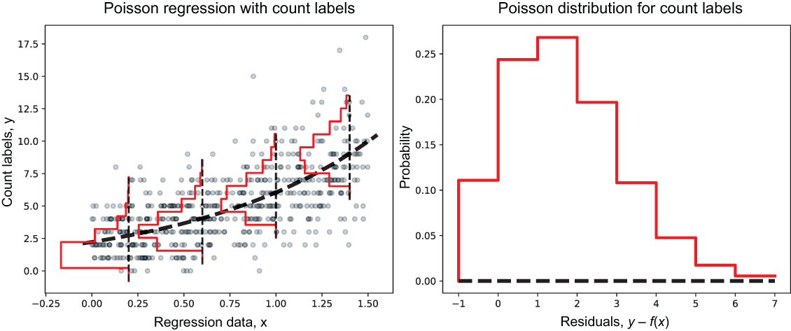
Compare the discrete Poisson spread used for count targets with the continuous normal spread assumed by linear regression. section 7.1.2
Choose the modeling assumptions around the observed count pattern:
- Use Poisson regression when the target is a count and a Poisson distribution is an appropriate model for its predictions. section 7.1.2
- Select a loss or negative log-likelihood consistent with the assumed target distribution; the choice changes how errors are penalized and the resulting model properties. section 7.3.1
- Adapt gradient boosting or Newton boosting through the loss function when fitting continuous or count-valued labels with sequential ensembles. section 7.3
- Consider a Tweedie distribution when counts contain many zeros and a long right tail, as it can represent a compound Poisson-gamma distribution. section 7.4.1
Predicting casual bike users
In the Bike Sharing data, the target casual ranges from 0 to 367. Its histogram has a large point mass at zero and a long right tail. Transforming labels as log(1 + y) avoids taking the logarithm of zero and suggests both a Tweedie distribution and, for a GLM formulation, a log-link function. Features are split into training and test sets, then normalized before evaluation. section 7.4.1
Figure 7.13 Histogram of count-valued targets, the number of casual users (left); histogram of the count targets after log transformation (right)
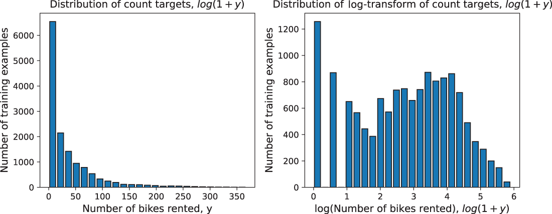
Inspect the raw and log-transformed bike-user counts to see the zero mass and right-skewed shape that affect distribution choice. section 7.4.1
For a direct baseline, scikit-learn's PoissonRegressor fits count targets and can be evaluated with mean squared error and mean absolute error. On the illustrated test split, Poisson regression reports lower MSE and MAD than ridge regression, though model selection should remain tied to the target distribution and problem setting. section 7.1.2

