A circuit-board layout turns components into vertices and conductive tracks into edges. Where tracks cross, the drawing may become less useful. For a graph G drawn in the plane, its crossing number cr(G) is the smallest number of edge crossings achievable across all its drawings—not merely the number in the layout currently on screen. A planar graph has crossing number 0; K5 and K3,3 each have crossing number 1. section 15.0 section 15.3
The allowed way of drawing edges matters:
- The crossing number permits plane drawings with curved edges. section 15.3.2
- The rectilinear crossing number rcr(G) restricts edges to straight-line segments, so rcr(G) cannot be smaller than cr(G). The two agree when cr(G) is at most 3, but can differ beyond that. section 15.3.2
A better drawing is not a different graph
A naïve drawing of K6 has 15 crossing pairs of edges; a minimum-crossing drawing has just 3 intersections. Moving the vertices and rerouting the edges changes the drawing, not the graph whose crossing number is being sought. section 15.3.1
Figure 15.14 The simplest graph for which the rectilinear crossing number is larger than the crossing number. Intersections are highlighted by the little arrows.
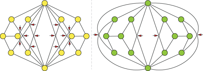
Compare the straight-line and curved-edge drawings: this graph has rectilinear crossing number 12 but crossing number 4. section 15.3.2
Finding the exact value for a general graph is NP-complete; an attractive drawing does not certify that its crossing count is minimal. There is a narrower test for a non-planar graph with crossing number 1: try each pair of non-adjacent edges, replace their proposed crossing with a new vertex joined to their four endpoints, and test the resulting graph for planarity. For broader layout problems, heuristics can seek drawings with fewer crossings without guaranteeing the minimum. The crossing count itself is a poor gradient-descent cost function because it creates plateaus and local minima; force-directed drawing instead optimizes layout quality and affects crossings indirectly. section 15.3.1 section 16.1 section 16.6
