The rectilinear crossing number rcr(G) is the minimum number of edge intersections among all drawings of graph G whose edges are straight-line segments. Restricting edges to segments can increase the minimum compared with the ordinary crossing number, which permits curves. section 15.3.2 section 16.1
The restriction has several useful consequences:
- rcr(G) is never smaller than the crossing number because straight-line drawings form only a subset of possible embeddings. section 15.3.2
- When the crossing number is at most 3, it matches the rectilinear crossing number; this equality does not extend to every graph. section 15.3.2
- Exact optimization is difficult, so randomized heuristics and simulated annealing search for low-intersection embeddings when guaranteed answers are impractical. section 16.1 section 17.3.1
Complete graphs and curved alternatives
For K8, the crossing number is 18 but rcr(K8) is 19. A simulated-annealing search reached an embedding with 19 crossings, whereas random sampling reached only 27 in the reported experiment. For some graphs, curved edges can achieve fewer crossings than any straight-line drawing. section 17.3.1 section 15.3.2
Figure 15.14 The simplest graph for which the rectilinear crossing number is larger than the crossing number. Intersections are highlighted by the little arrows.
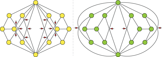
Compare a straight-line embedding realizing a larger rectilinear crossing number with a curved-edge embedding realizing the smaller ordinary crossing number. section 15.3.2
Figure 17.14 Two embeddings of complete graph K8. On the left, one was computed by the random sampling algorithm; on the right is the result of simulated annealing. Both algorithms were run for 500 iterations: random sampling could only get as low as 27 intersections, but simulated annealing produced an optimal embedding with 19 crossing points.
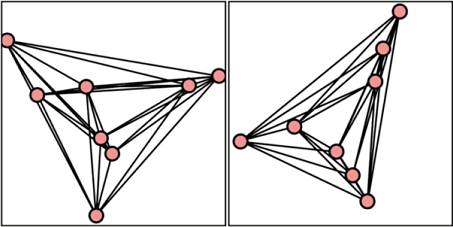
Inspect random sampling and simulated annealing results for K8, including the 27-crossing and 19-crossing embeddings. section 17.3.1
