Recurrent neural networks could carry information through a speech sequence, but training them effectively was difficult. Baidu’s Deep Speech 2 (DS2), reported in 2015, showed what large-scale, GPU-powered training could make practical: an end-to-end neural system that challenged traditional speech-recognition pipelines. Its achievement was less a single new trick than a combination of architecture, data, compute, and careful engineering. section 4.0 section 4.4 section 4.4.5
Older pipelines needed handcrafted phonetic dictionaries and precise labels marking where words began and ended in audio. DS2 instead learns from audio features to written symbols, using Connectionist Temporal Classification (CTC) to train without those frame-level alignments. It removes two labor-intensive parts of the pipeline, though it does not remove every external component. section 4.4.1 section 4.4.4
A recording passes through a sequence of stages:
- A spectrogram represents how sound energy changes over time; convolutional layers pick out local patterns. section 4.4.1
- Recurrent layers follow sounds across time. Early convolutional strides reduce the amount of sequence data they must process. section 4.4.1
- A final layer predicts English letter pairs or Mandarin characters. Row convolution adds a narrow window of temporal context to unidirectional outputs, trading some of a bidirectional model’s broader context for lower streaming latency. section 4.4.1
Figure 4.5 Left: DS2 architecture used to train on English and Mandarin speech. The authors vary the number of convolutional layers from 1 to 3 and the number of recurrent layers from 1 to 7. Right: structure of the RNN model from the first Deep Speech paper [45]. Used with permission granted by one of the authors (Awni Hannun).
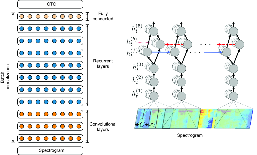
Compare the English-and-Mandarin DS2 architecture with the earlier Deep Speech RNN; the depicted DS2 variants use one to three convolutional layers and one to seven recurrent layers. section 4.4.1
Scaling the system required work beyond model design. Data parallelism split each batch across GPUs and synchronized their gradients; a custom GPU-to-GPU all-reduce made a training epoch 2.5 times faster than an off-the-shelf OpenMPI setup. Typical runs used 8–16 GPUs. For inference, half-precision (FP16) arithmetic roughly halved memory use and doubled throughput on compatible hardware without a significant accuracy loss. Optimized kernels and batch dispatch also helped deliver real-time transcription with median latency below 70 milliseconds. section 4.4.2 section 4.4.4
Where “human-level” depended on the test
On the WSJ eval’92 read-speech set, DS2’s word error rate was 3.60 versus 5.03 for human transcription. On noisy CHiME recordings, it was 21.79 versus 11.84. The comparison also drew criticism because some human benchmarks used nonexpert transcripts without further correction. DS2’s results were substantial, but not a blanket claim that it surpassed expert listeners in every setting. section 4.4.2 section 4.4.4
DS2 still used an external language model during beam-search decoding to choose plausible word sequences and correct phonetic errors. It was therefore a major step toward end-to-end recognition, not a system in which one network handled every part. Its lasting engineering lesson is that practical gains can come from fitting learning methods, computation, and deployment constraints together. section 4.4.4 section 4.4.5
