Derivative

As explained in Geometry for Programmers

A derivative measures the rate of change of a function with respect to an input variable.

A derivative measures how fast a function changes with its input. For a graph, it is the slope of the tangent line at a point: positive means the function is rising, negative means it is falling, and zero means it is momentarily flat. This turns a visual judgment about a curve into a number that code can use. section 5.1 section 5.1.1

Figure 5.3 As the interval decreases, the hypotenuse line becomes more like the tangent line.

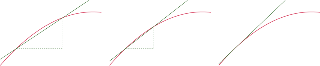
Shrinking the interval makes an average-change line approach the tangent line, revealing the derivative as local slope. section 5.1.1

At one input, a derivative is a number. Across a domain, those numbers form a new function, written with a prime when the variable is clear. A linear function has a constant derivative; differentiating a quadratic produces a linear function, and differentiating a cubic produces a quadratic. A function is differentiable at a point only when this measurement can be taken there. section 5.1.1 section 5.1.2

Useful differentiation rules let large expressions be handled in smaller pieces:

• A constant differentiates to 0, and a constant factor remains a factor. section 5.1.3
• A sum differentiates term by term; for polynomials, apply the power rule to each term. section 5.1.3 section 6.1.2
• A product uses f′g + fg′; nested functions use the derivative of the outer function times the derivative of the inner one. section 5.1.3

Finding the turning behavior of a polynomial

For P(x) = x³ − x² − 2x + 1, the derivative is P′(x) = 3x² − 2x − 2. Where a continuous derivative changes from positive to negative or back, the original polynomial changes from rising to falling or vice versa, producing a local maximum or minimum. A derivative root alone is not enough: if it touches the axis without changing sign, there need not be an extremum. section 6.1.2

Derivatives also describe geometric constraints. The derivative of a polynomial at a point gives the slope of its tangent, so interpolation equations can require a curve both to pass through chosen points and to leave them at chosen angles. Matching first derivatives where curve pieces meet supports smooth joins. A second derivative is connected to curvature, and continuity of successive derivatives describes levels such as C1 and C2 smoothness. section 7.1.1 section 5.6

For symbolic work, use SymPy’s diff to compute derivatives and select differentiation variables when needed. This leaves attention for interpreting slopes, smoothness, and curve behavior rather than memorizing every formula. section 5.1.5

How Geometry for Programmers covers it

How deep it goes

Explains tangent-line intuition, derivative functions, standard rules, higher derivatives, and symbolic computation, while deferring broader calculus applications.

Examples

Illustrates linear, quadratic, cubic, sine, and cosine derivatives, plus a cubic polynomial used to locate extrema.

What it assumes

Teaches derivatives from graph-based intuition while assuming comfort with functions, lines, and basic polynomial notation.

What you can do after

Apply it via SymPy to differentiate functions and interpret slopes, extrema, tangent constraints, and curve smoothness.

How it connects

Connects derivatives to tangent lines, parametric curves, curvature, smoothness, polynomials, splines, interpolation, and integration.

liveBookmanning.com

Read Geometry for Programmers on liveBook Get the book at manning.com

Also explained in

• 

  liveBookmanning.com
  Grokking AI Algorithms, Second EditionA derivative is a mathematical quantity that measures the instantaneous rate of change of a function with respect to its input.
• 

  liveBookmanning.com
  Deep Learning with R, Third EditionA derivative is a measure of how a function's output changes in response to an infinitesimal change in an input.
• 

  liveBookmanning.com
  Deep Learning with Python, Third EditionThe mathematical process of computing derivatives, used here to support gradient-based learning.
• 

  liveBookmanning.com
  Deep Learning with PyTorch, Second EditionA quantity describing how a function changes with respect to an input or parameter.
• 

  liveBookmanning.com
  Advanced Algorithms and Data StructuresA derivative measures the instantaneous rate at which a function changes with respect to its input.

Compare how 6 books explain derivative →

Related concepts

• differentiationproduced by · Differentiation is the mathematical operation of determining a function’s rate of change with respect to its inputs.
• gradient descentused by · Gradient descent is an iterative optimization method that updates parameters opposite the gradient of an objective function to reduce its value.
• slopemeasures · Slope is the rate at which a dependent quantity changes relative to an independent quantity, often represented by a line’s gradient or a coefficient in a linear relationship.
• backpropagationused by · Backpropagation is a procedure for computing derivatives of an output or loss with respect to inputs and parameters by applying the chain rule backward through a computational graph.
• gradientincludes · A gradient is the vector of partial derivatives of a scalar function with respect to its variables, indicating its local rate and direction of change.
• second derivativeincludes · A second derivative is the derivative of a function’s first derivative with respect to the same variable, describing how its rate of change varies.

This explainer was generated by Manning's knowledge graph from the text of Geometry for Programmers. The section links point to the parts of the book it draws on.