An ensemble combines several outlier detectors to produce a final score or label for each record. No single detector finds every kind of anomaly: different approaches may flag different records. Combining them can broaden coverage and make scores less dependent on one detector’s tendency to under- or overscore a record. It does not make every flagged record a meaningful anomaly. section 4.13 section 14.0
Build an ensemble in four steps:
- Test candidate combinations of detector, features, preprocessing, and parameters; retain their per-record scores. section 14.1
- Select reasonably accurate detectors that complement one another. Compare their highest-scored records: low correlation can indicate useful diversity, but an inaccurate detector can also be uncorrelated. section 8.4 section 14.4.5
- Make score direction and scale comparable where needed. Different detector types can produce dramatically different ranges; similarly configured instances of one type may be an exception to scaling. section 14.1 section 14.5
- Combine the scores into one score per record, then evaluate the complete combination rather than assuming the best individual detectors make the best ensemble. section 14.1 section 14.2
Diversity need not come only from changing algorithms. Vary missing-value handling, encoding, scaling, dimensionality reduction, or hyperparameters; train on different feature subsets or row samples. Feature subsets can expose anomalies hidden when irrelevant features are included, while row sampling offers different reference distributions. Very small samples may increase diversity at the cost of weaker individual detectors. section 14.3 section 14.3.2 section 14.3.4 section 14.3.6
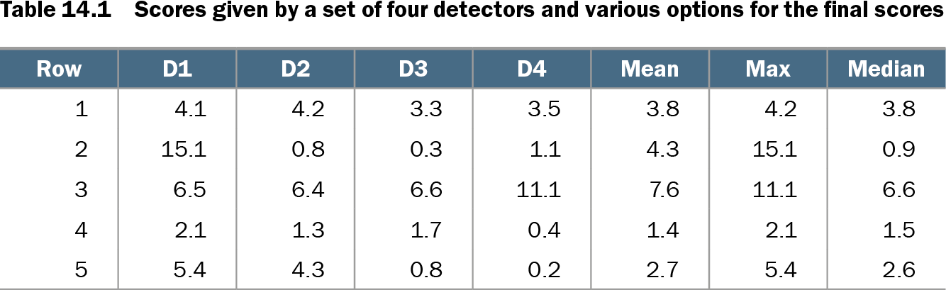
Choose the combining rule to match the desired behavior. A maximum retains a record flagged strongly in even one feature subspace; a mean smooths variation across parameter settings or row samples. Means can dilute isolated high scores and give correlated detectors disproportionate influence. A percentile or mean of the top few scores provides an intermediate choice between broad consensus and a single strong signal. None is universally best. section 14.6.1 section 14.6.3
Six views of baseball records
After imputing a missing field, encoding categories, and robustly scaling the baseball data, six detector types score the records. Isolation Forest scores lie around 0.3–0.7, while Elliptic Envelope scores span roughly 0–1000. Robustly scaling each score column before summing prevents the raw ranges alone from determining the final ranking. section 14.1 section 14.5
Table 14.1 Scores given by a set of four detectors and various options for the final scores (view table figure)
| Row |
D1 |
D2 |
D3 |
D4 |
Mean |
Max |
Median |
|---|---|---|---|---|---|---|---|
| 1 |
4.1 |
4.2 |
3.3 |
3.5 |
3.8 |
4.2 |
3.8 |
| 2 |
15.1 |
0.8 |
0.3 |
1.1 |
4.3 |
15.1 |
0.9 |
| 3 |
6.5 |
6.4 |
6.6 |
11.1 |
7.6 |
11.1 |
6.6 |
| 4 |
2.1 |
1.3 |
1.7 |
0.4 |
1.4 |
2.1 |
1.5 |
| 5 |
5.4 |
4.3 |
0.8 |
0.2 |
2.7 |
5.4 |
2.6 |
Compare mean, maximum, and median on the same four detector scores. A record with one score of 15.1 but three near 1 receives a maximum of 15.1 and a median of 0.9: the rule changes which records attract attention. section 14.6.1
Select a combination with a relevant metric, such as AUROC or precision at k, using labeled data when sufficient labels exist or a synthetic test set otherwise. A consensus score can serve as a pseudo-ground truth for choosing a smaller, cheaper ensemble, but its quality rests on the detectors being reasonably effective. Revisit the selection, scaling, and combining choices as an iterative process. section 14.2 section 14.4.2 section 14.7